

Антенны, СВЧ / OC / Должиков / Introduction to Smart Antennas_Balanis
.pdfINTEGRATION AND SIMULATION OF SMART ANTENNAS 123
antenna pattern (−26 dB sidelobes), which does not have an adaptive null toward the SNOI. From this figure, it can be concluded that the adaptive LMS beamforming algorithm leads to higher throughput by suppressing the interference (placing a null toward the SNOI) while the Tschebyscheff pattern does not have a null toward the SNOI.
7.7DISCUSSION
From the results obtained, it is possible to provide certain guidelines for the design of smart antenna systems for optimum capacity in MANETs. Antenna parameters, such as array size and excitation distribution, can be chosen to meet the capacity requirements for a network, based on the simulation results. From these simulation results, it can be concluded that:
(1)radiation patterns with smaller beamwidths result in higher network capacity,
(2)radiation patterns with lower sidelobes can further improve network capacity, and
(3)adaptive radiation patterns (i.e., capable of placing nulls toward the SNOIs) usually produce higher network capacity compared to patterns with lower sidelobes but no nulls toward the SNOIs.
Also, since there is a tradeoff between the network capacity and the training packet length, these simulations assist in choosing a suitable value for the training packet length without compromising on the network capacity. The training period places an upper bound on the convergence speed of the beamforming and DOA estimation algorithms, serving as a guideline for the algorithm design. The results show that training periods greater than 20% reduce the throughput considerably; therefore, it can be inferred that fast beamforming algorithms are critical for high-network capacity.
Employment of smart antenna systems in MANETs creates a wide scope for enhancing the network capacity. Through the design of efficient channel access protocols, spatial diversity of smart antennas can be exploited to increase the capacity of an ad hoc network. However, the design of such protocols requires a careful consideration of the system aspects of the smart antenna technology. In this work, a channel access protocol is suggested for MANETs employing smart antennas to communicate. This protocol is built based on the MAC protocol of IEEE 802.11 WLANs [175, 192] for TDMA environment. The protocol facilitates the use of smart antennas and decreases cochannel interference, thereby increasing the capacity of the network.
Finally, it has been shown that in slow fading channels, the performance of the DMI and LMS algorithms is similar. However, in fast fading channels the LMS algorithm is not as effective. Therefore, in such cases, it is suggested to initially use the DMI algorithm in

124 INTRODUCTION TO SMART ANTENNAS
acquisition and then use the LMS algorithm in the tracking mode. Furthermore, the system performance is improved when TCM is combined with antenna diversity.

125
C H A P T E R 8
Space–Time Processing
Space–time processing (STP) has become one of the most investigated technologies in wireless communications as it provides solutions to wireless environment problems such as interference, bandwidth, and range [25]. In this chapter we present the general principles of STP and demonstrate the major benefits from its applications.
8.1INTRODUCTION
STP signifies the signal processing performed on a system consisting of several antenna elements, whose signals are processed adaptively in order to exploit the rich structure of the radio channel in both the spatial (space) and temporal (time) dimensions. STP techniques can be applied either to the transmitter or the receiver, or both. Fig. 8.1 illustrates different link structures depending on the number of antennas used in receiving or transmitting modes. These options can be associated with both uplink and downlink. Depending on the number of antennas, the channel is classified as single input (SI) or multiple input (MI) for transmit and single output (SO) or multiple output (MO).
When STP is applied at only one end of the link, it is usually referred to as a smart antenna technique. When STP is applied at both the transmitter and the receiver, MIMO (multiple input, multiple output) techniques are used. Smart antenna and MIMO technologies have emerged as the most promising area of research and development in wireless communications, and they are capable of resolving the capacity limitations due to traffic congestions in future high-speed broadband wireless access networks [25].
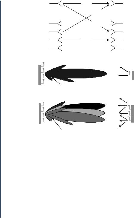
It has been recently shown that, under Rayleigh fading, the capacity of a multiple-antenna link increases almost linearly with the number of transmitting antennas provided that there are at least as many receiving antennas as transmitting antennas and the channel gain between each transmitting/receiving antenna pair is known to the receiver [195, 196]. To achieve this intended increase in capacity, various space–time coding schemes have been developed [197, 198]. Fig. 8.2 is an intuitive illustration of this advancement MIMO systems provide. In Fig. 8.2(a) an uplink system is illustrated with multiple antennas at the BS and a single antenna at the MS. The MS radiates omnidirectionally, while the BS is able to adapt its antenna pattern
126 INTRODUCTION TO SMART ANTENNAS
Tx |
SISO |
|
Rx |
|
|
|
O |
|
|
S |
|
|
|
I |
|
|
|
M |
|
|
|
SI |
|
|
|
M |
|
|
|
|
O |
Tx |
|
|
Rx |
|
MIMO |
|
|
FIGURE 8.1: Link structure [194].
 MS
MS
BS |
Nulls for interference rejection |
(a)
BS |
MS |
Nulls for rejecting undesired signal streams
(b)
FIGURE 8.2: Uplink antenna systems (a) BS with multiple antennas and MS with single antenna and
(b) MIMO system with multiple antennas at both the BS and MS [1].
and focus it into the MS while also rejecting interference through pattern nulls. In a practical scenario, the desired and interfering signals are likely to arrive from many different directions, and therefore the actual beam pattern may appear completely different and not reflect a focusing spatial filtering process [1]. In Fig. 8.2(b), a MIMO system is depicted where both the BS and MS are equipped with multiple antennas and several data streams are sent simultaneously over the wireless channel. Each antenna at the MS transmits a different data stream and radiates them omnidirectionally. At the BS, the antenna is capable of forming several beams that can select each of the data streams and correctly receive them. It is clear from this example that the capacity of the system has been significantly increased compared to a conventional system, and it justifies the excitement MIMO systems are generating [28].

SPACE–TIME PROCESSING 127
Due to the computationally intensive STP algorithms and the limited battery and processing capabilities of handheld mobile devices, until now almost all STP technology development has been related only to base stations and access points. However, with current advancements in low-power mobile device technology and ground-breaking innovation in STP techniques, this technology can also be applied to mobile devices.
Smart antenna technology is an attractive technique that increases spectrum efficiency, range and reliability of wireless networks. Systems that incorporate smart antennas usually have an array of multiple antennas only at one end of the communications link, for example, at the transmit side, such as MISO (multiple input, single output) systems; or at the receive side, such as SIMO (single input, multiple output) systems. Most conventional smart antenna systems employ the beamforming concept where the signal energy is focused in a particular direction (usually toward the receiver) to increase the received signal-to-noise ratio (SNR). Narrow antenna beams also reduce interference, improving signal to interference noise ratio (SINR) and thereby increasing the efficiency in spectrum management. Other smart antenna schemes improve the link quality by taking advantage of the diversity gain offered by multiple transmitting antennas.
When multiple antenna elements are used, the probability of losing a transmitted signal decreases exponentially with the number of decorrelated signals (or antennas). The diversity scheme used in current SIMO (or MISO) wireless LAN (WLAN) systems incorporates a simple switching network to select, out of an array of two antennas, the antenna that yields the highest SNR. MIMO systems can turn multipath propagation, usually harmful in wireless transmission, into an advantage for increasing the user’s data rate.
Diversity-based and smart antenna schemes do not increase the maximum data rate or significantly extend the range of operation; they simply improve the link quality and the efficient use of the spectrum. In contrast, the capacity of MIMO systems, in which antenna arrays are deployed at both the transmitter and the receiver, far exceeds that of conventional smart antennas [25].
In a multipath fading environment, the transmitted signal is reflected by various objects such as walls, buildings, trees and mountains before reaching the receiver. MIMO antenna techniques, accompanied with space–time processing, exploit rich scattering environments by sending independent data streams out of all the transmitting antennas simultaneously and in the same frequency band.
For example, a MIMO-based WLAN 802.11 system with four transmitting and four receiving antennas leads to a fourfold capacity gain up to 216 Mbits/s (4 × 54 Mbits/s), which can be shared by multiple hotspot users [25]. This type of MIMO technique is referred to as spatial multiplexing (SM). Depending on the environmental conditions experienced by the mobile device, the performance improvement of MIMO systems can be applied in two ways.
128 INTRODUCTION TO SMART ANTENNAS
When the channel conditions and SNR are favorable, the SM technique is used to increase the data rate [25]. In this case, the receiver expends some (if not all, depending on the STP algorithm used) of its degrees of freedom on retrieving the multiple signals rather than providing diversity against fading. However, at longer distances, multiple transmitting and receiving antennas are used to provide diversity and array gain for increased range. Depending on the channel conditions, a link adaptation algorithm, usually residing in the media-access controller (MAC) processor, provides the switching between diversity and SM modes of operation. Robust implementation necessitates the ability to adapt to the surrounding environment.
Depending on the propagation channel conditions and STP technique implemented, an N-fold, where N is the number of antennas on the transmitting and receiving ends, MIMO system can yield up to an N-fold capacity increase over that of a single-input, single-output (SISO) system.
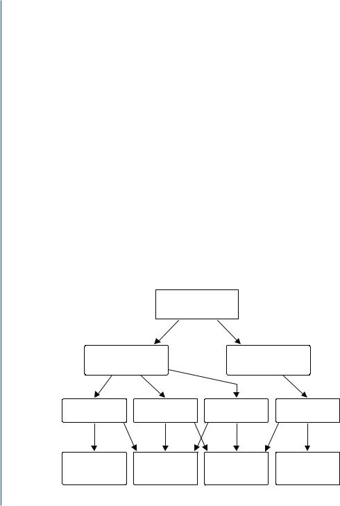
When signals are coherently combined at the receiver using techniques such as maximal ratio combining (MRC), the average received SNR increases by 10 · log10(N), where N is the number of receive antennas [25]. Obviously, there is a 6 dB improvement with a four-antenna solution. Fig. 8.3 illustrates the applications and benefits of STP.
In interference-cancelling MIMO systems, it is better to have more receiving antennas than transmitting. For example, if the number of transmitting antennas in a MIMO system is N, in order to cancel one interfering spatial multiplexing user with N independent data
space-time processing
smart antennas |
|
MIMO |
||
MISO/SIMO |
|
|
||
|
|
|
||
array gain |
interference |
diversity |
multiplexing |
|
reduction |
||||
|
|
|
||
coverage |
link quality |
capacity |
data rate |
(square miles/ |
(BER; outage |
(Erlangs/Hz/ |
(bits/second/Hz/ |
base station) |
probability) |
base station) |
base station) |
FIGURE 8.3: Space–time processing; applications and benefits [25].

SPACE–TIME PROCESSING 129
streams, the preferred number of receiving antennas is 2N. Each interfering multiplexing data stream is seen at the interference-cancelling MIMO receiver as a separate interferer. Therefore, N antennas are used to cancel the interference, and the remaining N antennas are used to demultiplex the desired data streams and achieve diversity gains.
The technique of joint spatial and temporal processing (an overview may be found in [27, 194]) was originally developed for multiuser wireless communications to provide cochannel interference mitigation. Later it was found that space–time processing can also be used to improve SNR, reduce the effect of multipath, provide diversity and increase array gain. In particular, the problem of blind space–time signal processing [199, 200] has gained significant attention in the recent years with the pioneering work on blind equalization using second-order statistics by Tong et al. [201] in 1994 and work on blind signal subspace based methods by Moulines et al. [202] in 1995 (the reader is also referred to [203, 204]). An elegant projection based solution to the multiuser blind equalization problem was proposed by Talwar [205, 206] for the ISI-free channel and Van der Veen [200] for the delay spread channel. The exploitation of the coding dimension in multichannel blind equalization still remains a promising and fertile area of research.
The first evidence of commercially successful small-form-factor multiple antenna technologies can be found in Japan with NTT Docomo’s personal digital cellular (PDC) and 3G Foma handsets, as well as in current 802.11 WLAN systems that use two diversity antennas at the receiving end. As described earlier, this technique does not increase the maximum data rate neither significantly extends the range of operation. However, it is a clear proof that multiple antenna technology is steadily penetrating the consumer product market. The biggest challenge to make STP technology commercially feasible is to make it affordable. To do this, both the signal processing algorithms and radio hardware must be implemented in a cost-effective manner. Solutions that can simultaneously integrate these aspects into next-generation silicon will become the key enabling technology for current and future generations of wireless systems. In what follows, an analysis of the space–time signal and channel models is reviewed that provides the necessary tools to examine the basic principles and unique advantages of space–time processing and beamforming afterwards. Finally, in this chapter results from several studies are incorporated which demonstrate the great benefits the wide employment of MIMO systems can yield.
8.2DISCRETE SPACE–TIME CHANNEL AND SIGNAL MODELS
To proceed with space-time processing, a discrete channel model is considered. This is derived by sampling the received signal in both space and time. The focus is initially drawn on the case of a single user transmitting a modulated signal in a specular multipath environment. At the transmitter, digital modulation is performed, a process by which a baseband signal is converted

130 INTRODUCTION TO SMART ANTENNAS
into an RF signal for transmission. Usually, the digital sequence {Ik } is linearly modulated by a pulse shaping function g (t) such that the baseband transmitted signal s (t) is represented in the general form
s (t) = |
∞ |
|
Ik g (t − kT) |
(8.1) |
|
|
k=−∞ |
|
where T is the symbol period. The data points Ik may come from any signal constellation (a set of vectors). For example, with BPSK the possible data symbols are two {±1}. In other modulations, such as QPSK or QAM, the sequence Ik is complex-valued, since the signal points have a two-dimensional representation. For the reader’s interest, the GSM system uses binary signals with GMSK (Gaussian Minimum Shift Keying) modulation for transmission over the air [207] (Ch. 6).
The fundamental function of a channel in signal processing and communications is to relate the transmitted signal to the received version of it [133]. For a baseband transmitted signal s (t), the received signal x(t) can be expressed as the convolution of the channel impulse response h(t, τ ) and s (t) as
x(t) = |
∞ |
|
h(τ, t)s (t − τ )d τ + n(t). |
(8.2) |
−∞
The impulse response h(τ, t) is a function of both the time delay τ introduced by the channel due to multipath propagation and the time t that accounts for the time evolution. Furthermore, additive noise n(t) is incorporated in (8.2). This is by far the most common assumption regarding noise, although other assumptions can be made as in [71, 72, 208].
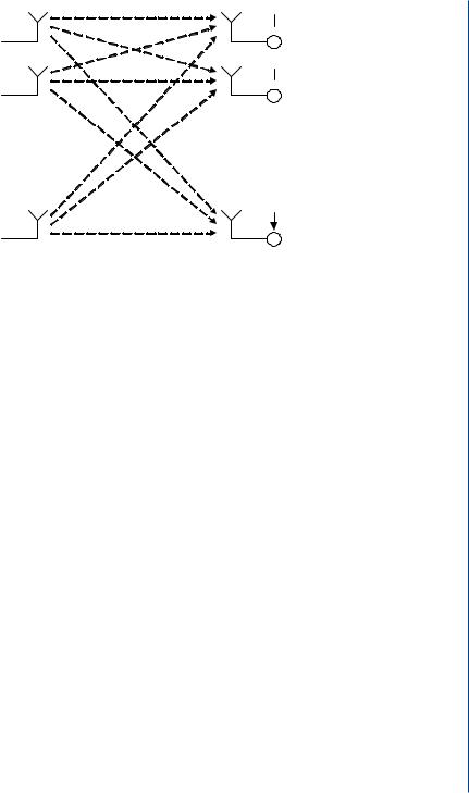
The previous expression for a single transmit and receive antenna is straightforwardly extended to the case of multiple antennas. For a communication link with N receive and M transmit antennas, the channel can be described by an N × M matrix H(τ, t) of complex baseband impulse responses. The element Hi j (τ, t) of the matrix denotes the impulse response from transmit antenna j to receive antenna i. That is, each receive antenna observes a noisy superposition of the M transmitted signals corrupted by the multipath fading channel. Hence, N M impulse responses are required to characterize this type of of Multi-Element Antenna (MEA) or MIMO channel. At each time instance, each row of H [Hi1, Hi2, . . . , Hi M] represents the channel’s response from the M transmitting to a single receiving element, whereas each column of H H1 j , H2 j , . . . , HN j represents the channel’s response from a single transmitting element to the N receiving antenna. The latter is also referred to as the spatio-temporal signature induced by the j th transmit antenna across the receive antenna array [209]. In principle, any channel model that accurately includes the spatial dimension can be used to investigate the correlation
SPACE–TIME PROCESSING 131
1
s1
2
s2
• • •
M
sM
H11
H21
HN 1
H12
H22
HN 2
H1M
H2M
HN M
n1
1
+ x1
x1
n2
2
+ x2
x2
• • •
nN
N
+  xN
xN
FIGURE 8.4: A wireless link comprising of M transmitting and N receiving antennas [70].
properties of two spatially separated antennas and derive the channel coefficients Hi j [133]. An excellent review is found in [210].
In the MEA case, and assuming that the channels between antenna pairs are independent and uncorrelated, the N × 1 vector of received signals x(t) becomes
∞ |
|
x(t) = H(τ, t)s(t − τ )dτ + n(t) |
(8.3) |
−∞
where s(t) denotes the M × 1 vector of transmitted signals and n(t) is the noise vector of the same length. A representation of the MEA channel is depicted in Fig. 8.4.
Here, it should be stressed that a continuous representation of the signals and impulse responses has been used which naturally arises when deriving the channel model from its physics and electromagnetics prospective [133]. However, most of the recent, and most likely future wireless communication systems employ digital signal processing to a large extent. When devising receiver structures and detector algorithms for these systems, it is more convenient to use a discrete time representation. With the received signal sampled with period T, the notation x(n) = x(nT) and
x(n) = |
∞ |
|
H(k, n)s(n − k) + n(n) |
(8.4) |
k=−∞
can be used. Note that H in (8.4) is the discrete time version of H in (8.3), as the sampled versions of the transmitted signal and the noise, denoted by s(n) and n(n), respectively, are further considered. This is the normal notation used in most of the literature, although the formulation results in some abuse of the notation. For narrowband systems, where the channel
132 INTRODUCTION TO SMART ANTENNAS
is considered to be frequency-flat, the main part of the received energy arrives at essentially the same time and the model may be further simplified to
x(n) = H(n)s(n) + n(n). |
(8.5) |
Here the channel model reduces to complex matrices comprising complex scalars that relate the received signals of each element to the corresponding transmitted signal from each antenna through a simple multiplying transfer matrix which encompasses the entire channel behavior. Further, if the channel is assumed to be time-invariant, the time dependency of the channel may be dropped, i.e. H. For this narrowband MIMO channel matrix, different normalizations
N |
M |
2 |
have been used in the literature, where the Euclidean or Frobenius norm H 2 = |
Hi j |
i=1 j =1
appears to be the most common one [211].
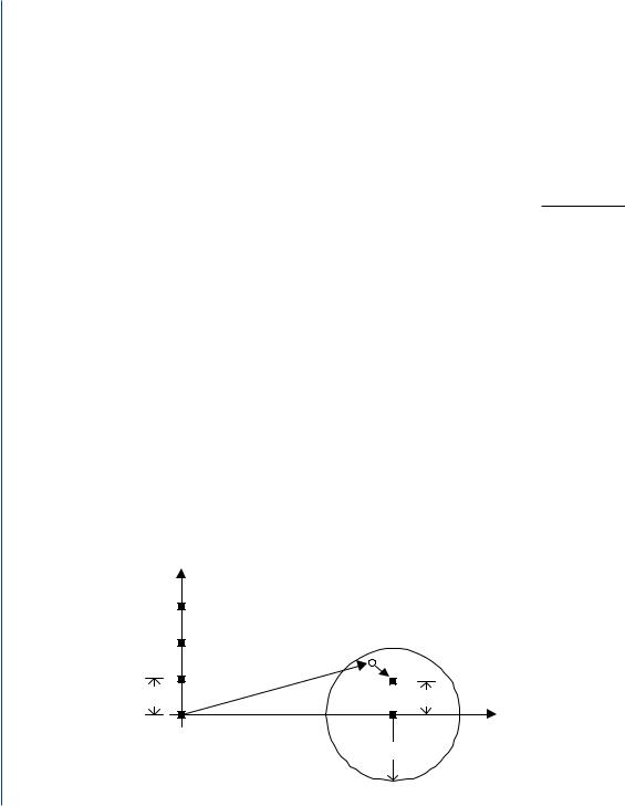
For the case of Rayleigh flat fading, a simple channel model assumes a circular disc of uniformly distributed scatterers placed around the mobile. In Fig. 8.5 a simple illustration of the scatter disc and the orientation of the mobile and base station are shown. Based on this model, the entries of the channel matrix in (8.5) are generated as follows. Assuming P scatterers Sp , p = 1, 2, . . . , P , are uniformly distributed on a disc of radius R centered around the mobile, the channel coefficient Hi j connecting the j th transmit to the ith receive antenna is given by
|
P |
2π |
|
|
|
Hi j = |
a p exp − j |
DB j →Sp + DSp →Mi |
(8.6) |
||
|
|||||
λ |
|||||
|
p=1 |
|
|
|
where DB j →Sp and DSp →Mi p, and scatterer p to the i
are the distances from the j antenna of the base station to scatterer antenna of the mobile unit, respectively. Also, a p is the scattering
Sp |
Sp |
DSp→Mi |
|
Mi |
|||
→ |
|
||
DBj |
|
||
dB |
|
dM |
|
Bj |
|
|
|
|
|
R |
|
FIGURE 8.5: Geometry of a channel [133]. |
|
|