-
The probability framework for statistical inference
-
Estimation
-
Testing
-
Confidence Intervals
Estimation
![]() is the natural estimator of
the mean. But:
is the natural estimator of
the mean. But:
-
What are the properties of
 ?
? -
Why should we use
 rather than some other estimator?
-
YB1B (the first observation)
-
maybe unequal weights – not simple average
-
median(YB1B,…, YBnB)
The
starting point is the sampling distribution of
![]() …
…
(a) The sampling
distribution of
![]()
![]() is a random variable, and its
properties are determined by the
sampling
distribution of
is a random variable, and its
properties are determined by the
sampling
distribution of
![]()
-
The individuals in the sample are drawn at random.
-
Thus the values of (YB1B,…, YBnB) are random
-
Thus functions of (YB1B,…, YBnB), such as
 ,
are random: had a different sample been drawn, they would have
taken on a different value
,
are random: had a different sample been drawn, they would have
taken on a different value -
The distribution of
 over different possible samples of size n
is called the sampling
distribution
of
over different possible samples of size n
is called the sampling
distribution
of
 .
. -
The mean and variance of
 are the mean and variance of its sampling distribution, E(
 )
and var(
)
and var( ).
). -
The concept of the sampling distribution underpins all of econometrics.
The sampling
distribution of
![]() ,
ctd.
,
ctd.
Example: Suppose Y takes on 0 or 1 (a Bernoulli random variable) with the probability distribution,
Pr[Y = 0] = .22, Pr(Y =1) = .78
Then
E(Y) = p1 + (1 – p)0 = p = .78
![]() = E[Y
– E(Y)]2
= p(1
– p)
[remember this?]
= E[Y
– E(Y)]2
= p(1
– p)
[remember this?]
= .78(1–.78) = 0.1716
The
sampling distribution of
![]() depends on n.
depends on n.
Consider
n
= 2. The sampling distribution of
![]() is,
is,
Pr(![]() = 0) = .222
= .0484
= 0) = .222
= .0484
Pr(![]() = ½) = 2.22.78
= .3432
= ½) = 2.22.78
= .3432
Pr(![]() = 1) = .782
= .6084
= 1) = .782
= .6084
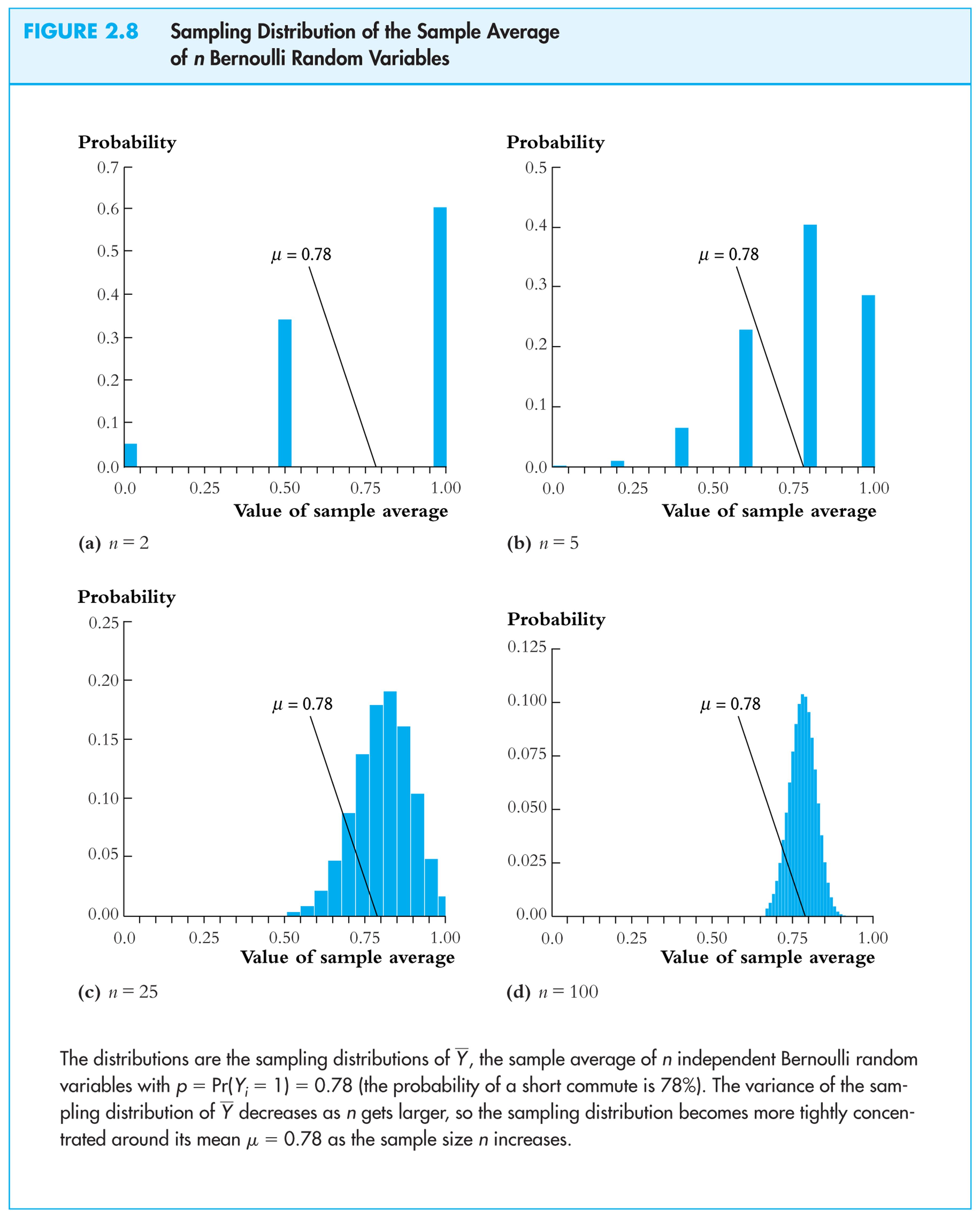
The sampling distribution of
![]() when Y
is Bernoulli (p
= .78):
when Y
is Bernoulli (p
= .78):
Things we want to know about the sampling distribution:
-
What is the mean of
 ?
?-
If E(
 )
= true
= .78, then
)
= true
= .78, then
 is an unbiased
estimator of
is an unbiased
estimator of
-
-
What is the variance of
 ?
?-
How does var(
 )
depend on n
(famous 1/n
formula)
)
depend on n
(famous 1/n
formula)
-
-
Does
 become close to
when n
is large?
become close to
when n
is large?-
Law of large numbers:
 is a consistent
estimator of
is a consistent
estimator of
-
-
 – appears bell shaped
for n
large…is this generally true?
– appears bell shaped
for n
large…is this generally true?-
In fact,
 –
is approximately normally distributed for n
large (Central Limit Theorem)
–
is approximately normally distributed for n
large (Central Limit Theorem)
-
The mean and variance of the sampling distribution of
General case – that is, for Yi i.i.d. from any distribution, not just Bernoulli:
mean:
E(![]() )
= E(
)
= E( )
=
)
=
 =
=
 = Y
= Y
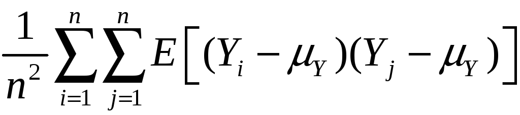
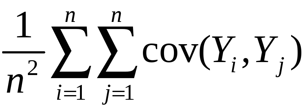
Variance:
var(![]() )
= E[
)
= E[![]() – E(
– E(![]() )]2
)]2
= E[![]() – Y]2
– Y]2
=
E
= E
so var(![]() )
= E
)
= E
=
=
=
=
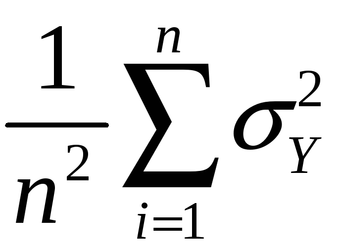
=
![]()
Mean and variance of
sampling distribution of
![]() ,
ctd.
,
ctd.
E(![]() )
= Y
)
= Y
var(![]() )
=
)
=
![]()
Implications:
-
 is an unbiased
estimator of Y
(that is, E(
is an unbiased
estimator of Y
(that is, E( )
= Y)
)
= Y) -
var(
 )
is inversely proportional to n
)
is inversely proportional to n
-
the spread of the sampling distribution is proportional to 1/

-
Thus the sampling uncertainty associated with
 is proportional to 1/
 (larger samples, less uncertainty, but square-root law)
The sampling distribution
of
![]() when n
is large
when n
is large
For
small sample sizes, the distribution of
![]() is complicated, but if n
is large, the sampling distribution is simple!
is complicated, but if n
is large, the sampling distribution is simple!
-
As n increases, the distribution of
 becomes more tightly centered around Y
(the Law of Large
Numbers)
becomes more tightly centered around Y
(the Law of Large
Numbers) -
Moreover, the distribution of
 –
Y
becomes
normal (the Central
Limit Theorem)
–
Y
becomes
normal (the Central
Limit Theorem)
The Law of Large Numbers:
An estimator is consistent if the probability that its falls within an interval of the true population value tends to one as the sample size increases.
If
(Y1,…,Yn)
are i.i.d. and
![]() < ,
then
< ,
then
![]() is a consistent estimator of Y,
that is,
is a consistent estimator of Y,
that is,
Pr[|![]() – Y|
< ]
1 as n
– Y|
< ]
1 as n
which
can be written,
![]()
![]() Y
Y
(“![]()
![]() Y”
means “
Y”
means “![]() converges in probability to
Y”).
converges in probability to
Y”).
(the
math: as n
,
var(![]() )
=
)
=
![]()
0, which implies that Pr[|
0, which implies that Pr[|![]() – Y|
< ]
1.)
– Y|
< ]
1.)
The Central Limit Theorem (CLT):
If (Y1,…,Yn)
are i.i.d. and 0 <
![]() < ,
then when n
is large the distribution of
< ,
then when n
is large the distribution of
![]() is well approximated by a normal distribution.
is well approximated by a normal distribution.
-
 is approximately distributed
N(Y,
is approximately distributed
N(Y,
 )
(“normal distribution with mean Y
and variance
)
(“normal distribution with mean Y
and variance
 /n”)
/n”) -
 (
( – Y)/Y
is approximately distributed N(0,1)
(standard normal)
– Y)/Y
is approximately distributed N(0,1)
(standard normal) -
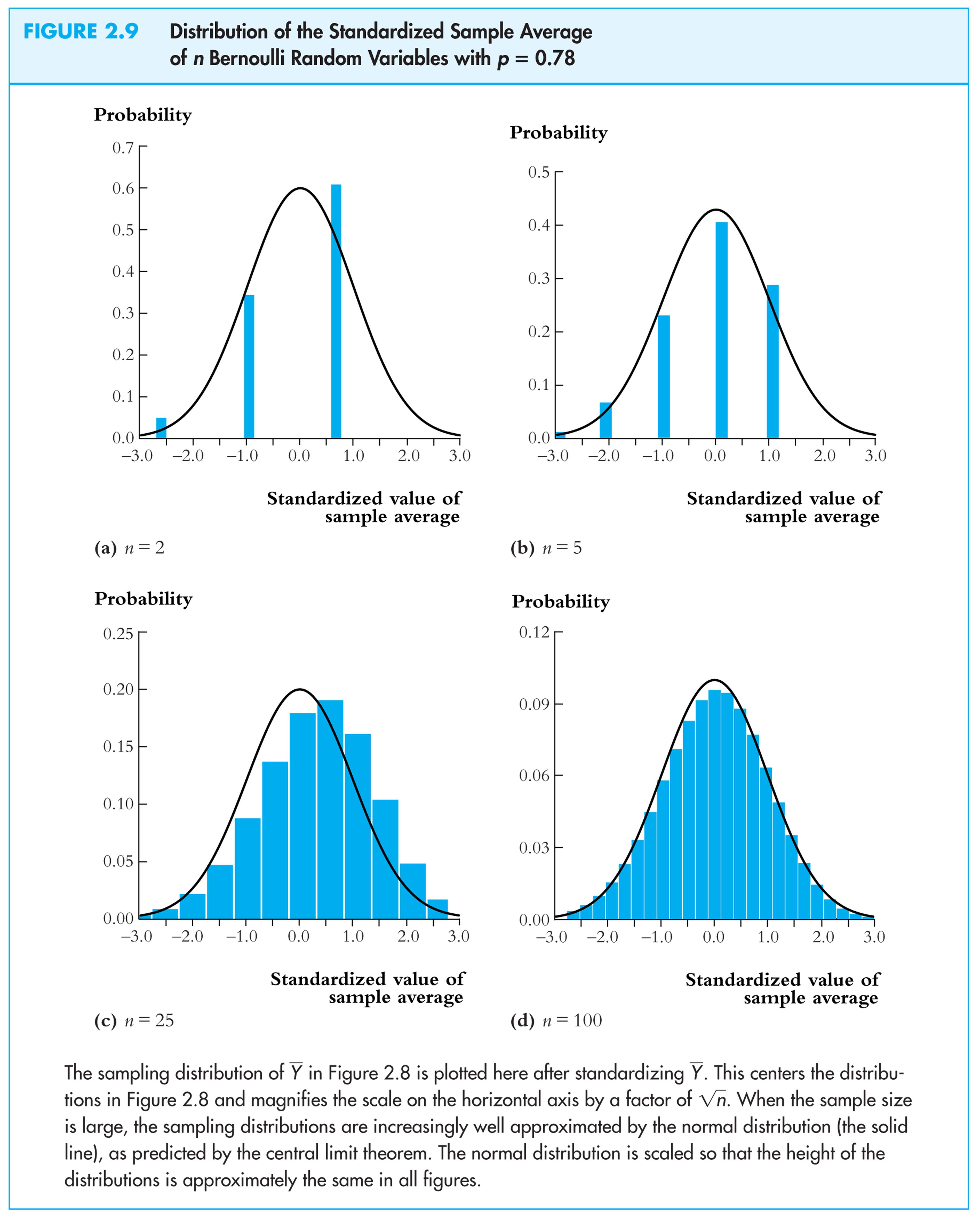
That is, “standardized”
 =
=
 =
=
 is approximately distributed as N(0,1)
 -
The larger is n, the better is the approximation.
Sampling distribution of
![]() when Y
is Bernoulli, p
= 0.78:
when Y
is Bernoulli, p
= 0.78:

Same example:
sampling distribution of
 :
: