

Chapter 9
Solving
Mathcad supports many functions for solving a single equation in one unknown through large systems of linear, nonlinear, and differential equations, with multiple unknowns. The techniques described here generate numeric solutions. Chapter 13, “Symbolic Calculation,” describes a variety of techniques for solving equations symbolically.
Solving and Optimization Functions
Finding Roots
Finding a Single Root
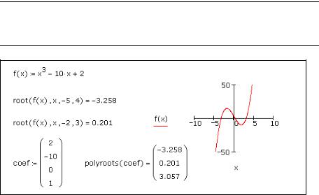
The root function solves a single equation in a single unknown, given a guess value for the unknown. Or, you can give root a range [a,b] in which the solution lies and no guess is required. The function returns the value of the unknown variable that makes the equation equal zero and lies in the specified range, by making successive estimates of the variable and calculating the value of the equation.
The guess value you supply for x becomes the starting point for successive approximations to the root value. If you wish to find a complex-valued root, start with a complex guess. When the magnitude of f(x) evaluated at the proposed root is less than the value of the tolerance parameter, TOL, Mathcad returns a result. Plotting the function is a good way to determine how many roots there are, where they are, and what initial guesses are likely to find them.
Tip As described in “Built-in Variables” on page 81, you can change the value of the tolerance, and hence the accuracy of the solution found by root, by including definitions for TOL in your worksheet. You can also change the tolerance by using the Built-in Variables tab when you choose Worksheet Options from the Tools menu.
Figure 9-1: Finding roots with root and polyroots.
103

104 / Chapter 9 Solving
Note When you specify the optional arguments a and b for the root function, Mathcad only finds a root for the function f if f(a) is positive and f(b) is negative or vice versa. (See Figure 9-1.)
If, after many approximations, Mathcad still cannot find an acceptable answer, it marks the root function with an error message indicating its inability to converge to a result.
To find the cause of the error, try plotting the expression. A plot helps to determine whether or not the expression crosses the x-axis and if so, approximately where. In general, the closer your initial guess is to where the expression crosses the x-axis, the more quickly the root function converges on an acceptable result.
Online Help For more details and issues on finding roots see “Finding Roots” in online Help.
The root function can solve only one equation in one unknown. To solve several equations simultaneously, use Find or Minerr described in “Solve Block Functions” on page 105.
Finding All Roots
To find the roots of a polynomial or an expression having the form:
vnxn + … + v2x2 + v1x + v0
you can use polyroots rather than root. polyroots does not require a guess value and returns all roots at once, whether real or complex. You must type the coefficients of the polynomial into a separate vector as in Figure 9-1.
Note root and polyroots can solve only one equation in one unknown and always return numerical answers. To solve an equation symbolically or to find an exact numerical answer in terms of elementary functions, use the solve keyword or choose Variable > Solve from the Symbolics menu. See Chapter 13, “Symbolic Calculation.”
Linear/Nonlinear System Solving and Optimization
Mathcad includes many other numerical solving functions.
Solving a Linear System of Equations
Use the lsolve function to solve a linear system of equations whose coefficients are arranged in a matrix M. The argument M for lsolve must be a matrix that is neither singular nor nearly singular. An alternative to lsolve is to solve a linear system by using matrix inversion.
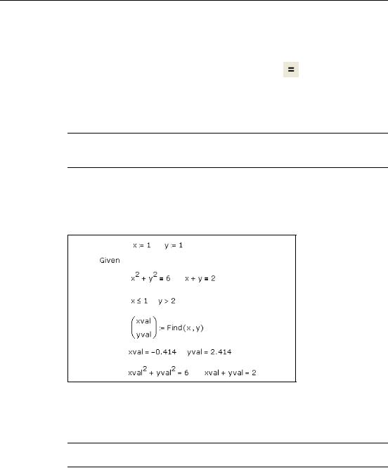
Solve Blocks
The general form for using system solving functions in Mathcad is within the body of a solve block. There are four steps to creating a solve block:
1.Provide an initial guess for each of the unknowns. Mathcad solves equations by making iterative calculations. The initial guesses give Mathcad a place to start searching for solutions. If you expect your solutions to be complex, provide complex guess values.
Solving and Optimization Functions / 105
2.Type the word Given in a separate math region below the guess definitions, in order to set up a system of constraint equations. Be sure you don’t type Given in a text region.
3.Now enter the constraints (equalities and inequalities) in any order below the word
Given. Make sure you use the Boolean equal symbol ( |
|
on the Boolean toolbar |
or press [Ctrl] [=]) for any equality. You can separate the left and right sides of |
||
an inequality with any of the symbols <, >, ≤, and ≥. |
|
|
4.Enter any equation that involves one of the functions Find, Maximize, Minimize, or Minerr below the constraints.
Tip Solve blocks cannot be nested inside each other — each solve block can have only one Given and one Find (or Maximize, Minimize, or Minerr). You can, however, define a function like f(x) := Find(x) at the end of one solve block and refer to this function in another solve block.
Solve Block Functions
Figure 9-2 shows a solve block with several kinds of constraints and ending with a call to the Find function. There are two unknowns. As a result, the Find function takes two arguments, x and y, and returns a vector with two elements.
Guess Values
Results
Check
Figure 9-2: A solve block with both equalities and inequalities. The equations for a circle and line are entered, then the inequality constraints are set. Find looks for the points of intersection, which are checked back in the original equations. See the QuickSheet “Solve Blocks with Inequality Constraints.”
Note Unlike most Mathcad functions, the solving functions Find, Maximize, Minerr, and Minimize can be entered in math regions with either an initial lowercase or an initial capital letter.
Solve blocks can be used to solve parametric systems. In Figure 9-3, the solution is cast in terms of several parameters in the solve block besides the unknown variable.
Solve blocks can also take matrices as unknowns and solve matrix equations. (See Figure 9-4 and Figure 9-5.)
106 / Chapter 9 Solving
Same problem, solved for a vector of answers...
Figure 9-3: Solving an equation parametrically.
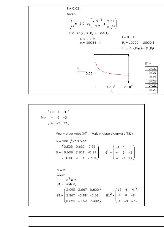
Two methods for computing a matrix square root (nonunique)
Using eigenanalysis:
Using a solve block: initial guess
Figure 9-4: A solve block for computing the square root of a matrix.
Note You can improve the solve block result in Figure 9-4, and those of many other sensitive problems, by decreasing the CTOL variable.
Solving and Optimization Functions / 107
State matrices:
Figure 9-5: A solve block for computing the solution of a matrix equation using the Riccati Equation from control theory.
Note Mathcad solve blocks can solve linear and nonlinear systems of up to 400 variables. The Solving and Optimization Extension Pack solves linear systems up to 1000 variables, nonlinear systems up to 250 variables, and quadratic systems up to 1000 variables.
The table below lists the constraints that can appear in a solve block between the keyword Given and the functions Find, Maximize, Minerr, and Minimize. x and y represent real-valued expressions, and z and w represent arbitrary expressions.
Constraints are often scalar expressions but can also be vector or array expressions.
Condition |
Boolean |
Constraint |
||
Toolbar |
||||
|
|
|||
w = z |
|
|
Equal |
|
|
|
|||
x < y |
|
|
Less than |
|
|
|
|||
|
|
|||
x > y |
|
|
Greater than |
|
|
|
|||
|
|
|||
x ≤ y |
|
|
Less than or equal to |
|
|
|
|||
|
|
|||
x ≥ y |
|
|
Greater than or equal to |
|
|
|
|||
|
|
|||
¬x |
|
|
Not |
|
|
|
|||
|
|
|||
x y |
|
|
And |
|
|
|
|||
|
|
|||
x y |
|
|
Or |
|
|
|
|||
|
|
|||
x y |
|
|
Xor (Exclusive Or) |
|
|
|
|||
|
|
|||
|
|
|
|
|
Mathcad does not allow the following between Given and Find in a solve block:
•Constraints with “≠.”
•Range variables or expressions involving range variables of any kind.
•Assignment statements (statements like x:=1).
You can include compound statements such as 1 ≤ x ≤ 3.
Note Mathcad returns only one solution for a solve block. There may, however, be multiple solutions to a set of equations. To find a different solution, try different guess values or enter an additional inequality constraint that the current solution does not satisfy.
108 / Chapter 9 Solving
Tolerances for Solving
Mathcad’s numerical solvers make use of two tolerance parameters in calculating solutions in solve blocks:
•Convergence tolerance. The solvers calculate successive estimates of the values of the solutions and return values when the two most recent estimates differ by less than the value of the built-in variable TOL. A smaller value of TOL often results in a more accurate solution, but the solution may take longer to calculate.
•Constraint tolerance. This parameter, the built-in variable CTOL, controls how closely a constraint must be met for a solution to be acceptable. For example, if the constraint tolerance were 0.0001, a constraint such as x < 2 would be considered satisfied if, in fact, the value of x satisfied x < 2.0001.
Procedures for modifying the values of these tolerances are described in “Built-in Variables” on page 81.
Online Help For more information on solving issues see “Find,” “Minerr” and “Solver Problems” in online Help.
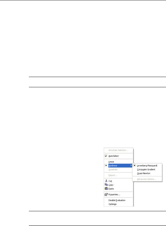
Solving Algorithms and AutoSelect
When you solve an equation, by default Mathcad uses an AutoSelect procedure to choose an appropriate solving algorithm. The available solving methods are:
•Linear. Applies a linear programming algorithm to the problem. Guess values for the unknowns are not required.
•Nonlinear. Applies either a conjugate gradient, Levenberg-Marquardt, or quasiNewton solving routine to the problem. Guess values for all unknowns must precede the solve block. Choose Nonlinear > Advanced Options from the menu to control settings for the conjugate gradient and quasi-Newton solvers.
To override Mathcad’s default choice of solving algorithm:
1.Create and evaluate a solve block, allowing Mathcad to AutoSelect an algorithm.
2.Right-click on the name of the function that terminates the solve block and remove the check from AutoSelect on the menu.
3.Check another solving method on the menu. Mathcad recalculates the solution using the method you selected.
Note When solving overdetermined systems, such as regression problems, the Levenberg-Marquardt method performs best if given a vector of residual values set to zero, rather than a single sum- of-squared errors objective function.