Учебники / Otolaryngology - Basic Science and Clinical Review

WHAT IS SOUND?

WHAT IS SOUND PRESSURE?

WHAT IS SOUND FREQUENCY?

TO WHAT SOUNDS ARE OUR EARS SENSITIVE?

INFLUENCES ON THE PROPAGATION OF SOUND

OF HUMAN PERCEPTION

THE SPEED OF SOUND C

SOUND WAVELENGTH AND THE DIFFRACTION

AND SCATTERING OF SOUND

VARIATIONS OF SOUND PRESSURE WITH

DISTANCE FROM A SOURCE

THE EAR AS A COLLECTOR OF SOUND

OVERVIEW

THE EXTERNAL EAR

THE TYMPANO-OSSICULAR SYSTEM

SOUND STIMULATION OF THE INNER EAR: OTHER PATHS FOR SOUND STIMULATION

THE ACOUSTICS AND MECHANICS OF

DISEASED MIDDLE EARS

OSSICULAR INTERRUPTION WITH AN INTACT

TYMPANIC MEMBRANE

LOSS OF THE TYMPANIC MEMBRANE, MALLEUS,

AND INCUS

OSSICULAR FIXATION

TYMPANIC MEMBRANE PERFORATION

MIDDLE EAR EFFUSION

THE ACOUSTICS AND MECHANICS OF RECONSTRUCTED

MIDDLE EARS

TYMPANOPLASTY TECHNIQUES WITHOUT OSSICULAR

LINKAGE: TYPES IV AND V

TYMPANOPLASTY TECHNIQUES WITH PRESERVATION OF OSSICULAR LINKAGE: TYPES I, II, AND III

CANAL WALL-UP VERSUS CANAL WALL-DOWN

MASTOIDECTOMY

STAPEDOTOMY

SUMMARY

SUGGESTED READINGS

SELF-TEST QUESTIONS

The physical properties that define how sound propagates in air are of great consequence in how we perceive sound.This chapter will review some of the elementary physical processes associated with sound propagation in

air and the reception of sound by human ears. The chapter is not meant to provide indepth details about physical processes of sound and its reception but is instead meant to impart some very basic perceptual

consequences of how sound propagates in air, how sound is collected by the ear, and how these processes are affected by pathology. Readers interested in a more detailed description of sound and the ear could read some elementary texts on the subject (see suggested readings,Yost, 1994).

WHAT IS SOUND?

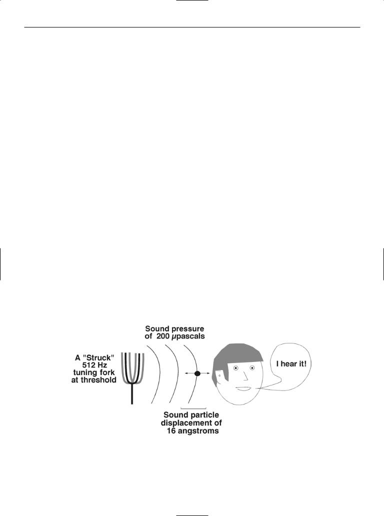
Sound results when particles of a medium are set into vibration. The sounds we hear, for the most part, result from air particles being set in motion by vibrating objects. For example, the vibrating tines of a struck 512 Hz tuning fork (Fig. 21-1) produce backward and forward motions of the air particles that surround the tines. (An air particle is a small volume of air that contains many air molecules.) The particles are set in motion by the vibrating tines, then push on the air particles next to them, where the push is proportional to the sound pressure, setting the next layer of particles into back-and-forth motion. The physical disturbance of sound pressure and particle motion, not the particles themselves, propagates through the air medium as succeeding layers of air particles are set into vibration.The amplitude of the propagating physical disturbance can be quantified in terms of either the sound pressure acting on the particles or the amplitude of the particle motions. The dependence of sound propagation on the presence of a medium explains why sound does not propagate through a vacuum.

A 512 Hz tone that is just audible to many humans will be associated with pressure variations of 0.2 millipascal

(a pascal is a unit of pressure, see later) and back-and-forth particle displacements of 16 angstroms (Å). In general, the louder the sound, the larger the particle motions and pressure variations. In practice it is easy to measure the pressure variations and more difficult to measure the motion of air particles, so sound pressure is the primary measure of sound amplitude.

WHAT IS SOUND PRESSURE?

Sound pressure refers to the magnitude of the cyclic variations in pressure produced around ambient static pressure when a sound is produced (Fig. 21-2).A pressure has units of force per area.The international unit of pressure is the pascal (Pa), where 1 Pa 1 newton (N) of force per square meter of area. A newton is the force necessary to accelerate a kilogram 1 m/s2.This is a moderate force, but the pressure produced by spreading a newton over a square meter of area is very small. In fact, 1 Pa of pressure equals only 1 10 5 atmospheres.The quietest sounds we hear are of even lower pressure; the change in pressure associated with sound at the threshold of hearing for a 1000 Hz tone is 20 micropascals ( Pa) or 2 10 10 atmospheres.

There are several ways to quantify sound pressure, though the most common is in terms of the root mean square (rms) deviation in pressure. Fig. 21-2A is an illustration of the changes in pressure with time that are associated with a 512 Hz tone.This figure illustrates the simple relationship between peak, peak-to-peak, and rms measures of amplitude of a pure tone where these different measures of amplitude yield values of 1, 2, or 0.71 Pa,

Figure 21-1 A struck tuning fork sets nearby air particles into motion with a frequency equal to the natural frequency of the fork. Associated with the motion of the air particles is a sound pressure. The air particles that are set in motion push on the particles next to them, and so forth, resulting in a propagating

physical disturbance. A tone of 512 Hz that is just audible is associated with air particles in free space moving back and forth with a magnitude of 16 angstroms (Å) (a displacement that is a little larger than the diameter of a hydrogen atom) and pressure oscillations of 200 micropascals ( Pa)

A

Figure 21-2 Two patterns of temporal variations in pressure in air produced by sound.The absolute value of the pressure is scaled in both plots,and therefore the sound-induced variations occur around a static value of 100,000 Pa 1 atmosphere.The sound pressure corresponds to the amplitude of the variations around the static value;in the illustrated cases, while the static atmospheric pressure is 100,000 Pa, the amplitude of the sound pressure is on the order of 1 Pa. (A) The pressure variations are those of a 512 Hz tone.The pressure varies sinusoidally with a period of 1/512 0.00195 sec.The amplitude of the pressure variation about the static value can be quantified in terms of: the peak-to-peak value of 2 Pa, the peak value of 1 Pa, or the root mean square (rms) value of 0.707 Pa rms.(The root mean square value

respectively.The time-varying sound pressure waveform illustrated in Fig. 21-2B is not readily quantified by peak measures but is well described by its rms value. In fact, the rms sound pressure of this complex sound is 0.71 Pa, a value identical to the tonal sound pressure observed in Fig. 21-2A.

The human auditory system is sensitive to a wide range of sound pressures:The minimum sound level that a human can hear is between 10 and 20 rms Pa. Conversational speech has pressures that are 100 times threshold. A lecturer or loud speaker will talk with sound pressures 1000 times threshold. Music often contains sound pressures that are 10,000 times threshold. Guns, fireworks, and jet engines can produce pressures that are more than 1,000,000 times threshold. Because of this sensitivity to pressures that vary by more than 1,000,000 times, and because our ear is generally sensitive to fractional changes in pressure, we commonly use

B

of the variation in pressure is the square root of the mean of the squared pressure deviations from static values averaged over some time. In the case of a sinusoid, a convenient averaging time is some integral number of periods of the sine wave.With sinusoidal sound pressures,the rms value equals the peak amplitude/ 2.) (B) The pressure variations are those of a complex sound with many irregular risings and fallings of the sound pressure.With this kind of sound, peak amplitude and peak-to-peak amplitude are poor indicators of the average sound level. However, rms is an excellent measure as long as one specifies an averaging time;in this case,we compute the rms sound pressure over the 0.01 sec time window shown in the illustration. Note that the sound pressure in B has the same rms value as the sound pressure in A.

a logarithmic scale to grade pressures.The decibel (dB) is a logarithmic measure of relative energy, where 10 dB (1 bell) represents an increase over a given reference energy level of one order of magnitude (i.e., one common log unit or a factor of 10).The common reference level for sound pressure level (SPL) is 2 10 5 Pa, and because energy is proportional to pressure squared:

where X is the sound pressure in rms pascals. Different dB sound pressure scales use different reference pressures [e.g., the dB hearing level scale (dB HL) of the

TABLE 21-1 THE SOUND PRESSURES OF COMMON SOUNDS

Approximate

Sound Level

dB, decibel; Pa, pascal; rms, root mean square; SPL, sound pressure level.

clinical audiogram uses the average sound pressure threshold of the normal population at a given frequency as the reference pressure].The SPL of both of the sounds in Fig. 21-2 is 91 dB SPL, where 91 20 log10 (0.71/0.00002). The sound pressures of various commonly experienced sounds are noted in terms of rms pascals and dB SPL in Table 21-1.

WHAT IS SOUND FREQUENCY?

Sound varies not only in amplitude but with time. One of the simpler sounds is a pure tone in which the relationship between time and sound pressure is described by a sine function, as in Fig. 21-2A, where the sound pressure, the variation in pressure about atmospheric pressure, equals sin(2 512t), where t is time in seconds. The human ear is sensitive to sound frequencies of 20 to 20,000 Hz. Complex sounds (e.g., Fig. 21-2B) can be described by the addition of pure tones of different frequencies and different phases. One can investigate the frequency content of sounds by using a Fourier spectrum analyzer that converts temporal responses into frequency spectra. Fig. 21-3 shows the spectra of the magnitudes of the two time waveforms of Fig. 21-2. The 512 Hz tone of Fig. 21-2A gives rise to a line spectrum at 512 Hz with no other spectral components. The magnitude of the sound pressure spectral component of the tone is 0.71 rms pascal (the lefthanded scale of Fig. 21-3) or 91 dB SPL (scaled on the right). The superimposed spectral analysis of the complex sound of Fig. 21-2B demonstrates that the sound is made up of multiple components with varied pressure magnitude.

It should be noted that although the spectra of Fig. 21-3 describe the magnitudes and frequencies of the different spectral components that make up the sounds of Fig. 21-2, the illustrated spectra do not contain enough information to reconstruct the

Figure 21-3 The Fourier spectra of the two sound signals from Fig. 21-2 are illustrated. The black line shows the line spectral magnitude at 512 Hz associated with the 512 Hz pure tone of Fig. 21-2A. The gray lines show the magnitudes of the spectral components of the complex sound of Fig.21-2B.The linearly scaled abscissa or horizontal axis describes the frequency of the different components. The logarithmically scaled left-hand vertical axis or ordinate describes the rms magnitude of the different spectral pressure components.The linear dB scale on the right calibrates the pressure magnitude of the components in terms of dB SPL.

waveforms of Fig. 21-2. What is missing is phase information.The phase of a sinusoid describes the time when the pressure crosses from negative to positive. This timing information is critical when we combine waves, because two waves added together can sum constructively if they have similar phases, sum to near 0 if the waves are out of phase and of identical magnitude, or anything in between. Many spectral analyzers also yield phase information.

TO WHAT SOUNDS ARE

OUR EARS SENSITIVE?

Every human ear is differentially sensitive to sounds of different frequency, but measurements of human sensitivity to sound vary depending on how we specify the sound stimulus. Fig. 21-4 compares two different measurements of the mean sound pressure threshold measured in normal young adults with pure tones of different frequencies. (The sound pressure threshold is the lowest sound pressure that is audible.) The lower curve in Fig. 21-4 depicts sound pressure measurements made with the listeners in an anechoic room where the sound pressure measurement was made where the listener’s head would be when the listener was not present (a “free field” description of the sound

Figure 21-4 The sensitivity of the ear to sounds of different frequencies. This figure is a comparison of two studies of auditory threshold, those combinations of sound pressure level and frequency that are just audible: The American National Standards Institute (ANSI) description (1969) of normal hearing threshold made under earphones and the free-field studies of Sivian and White (1933) made in an anechoic room.The sound pressure scale on the ordinate is in units of dB SPL. Frequency, on the abscissa, is plotted on a log scale.The mean normal threshold at 1000 Hz in both measurement conditions is 0 dB SPL.

pressure). The upper curve is the American National Standards Institute (ANSI) standard measurement of human thresholds made under earphones, where the sound pressures are those generated by the earphones in a calibration coupler. The differences between these two thresholds can be explained by the

effect of the human listener on the open sound field, the effect of closing the ear canal by earphones, and differences in calibration between the two circumstance (Shaw, 1974).

Whether under earphones or in the “free field,” however, it is clear that normal young adult humans are most sensitive to sound frequencies of 500 to 8000 Hz.The best frequency differs depending on the measurement circumstance, being equal to 1500 Hz under earphones and 4000 Hz in the free field. At higher and lower frequencies, more sound pressure is required to induce a threshold response, and the thresholds move up steeply below 500 Hz and above 8000 Hz.

Otologists and audiologists are usually most interested in how measurements of an individual’s hearing thresholds differ from normal, where under earphones normal is practically defined by the ANSI standard measurements of Fig. 21-4. The most powerful graphical tool for comparing two different functions is to plot their difference. The clinical audiogram (Fig. 21-5) uses this difference technique by plotting the individually determined sound threshold relative to the ANSI normal hearing level. For example, a person who is shown to have a hearing threshold at 1000 Hz of 10 dB greater than the ANSI standard would be assigned a hearing level of 10 dB at that frequency. In clinical audiograms, sound pressure relative to the standard is plotted on a decreasing scale in dB relative to normal, and frequency is tested in octave or halfoctave intervals. Remember that the normal curve is based on mean thresholds and that there is normal variation about the mean.

Figure 21-5 The clinical audiogram.The sound pressure scale is relative to the ANSI standard description of normal human hearing thresholds, and the scale is inverted so that higher thresholds are plotted lower on the graph. The gray-shaded region shows the range of variations in normal listeners.

INFLUENCES OF THE

PROPAGATION OF SOUND

ON HUMAN PERCEPTION

THE SPEED OF SOUND C

The sound-induced vibration of particles propagates through space by pushing on other particles and setting them into vibration. The velocity of propagation of sound through a medium is proportional to the root of the stiffness of the medium (the pressure necessary to change the volume by a set amount) and inversely proportional to the root of the density (mass per unit volume) of the medium. Table 21-2 compares the stiffness, density, and speed of sound in air, water, and hydrogen.The gases have a similar low stiffness compared with water, and the density varies greatly among the three media. Comparison of the entries in Table 21-2 argues against the common misconception that sound travels faster in water because water is more dense. In fact, sound travels faster in water because water is much stiffer than air; the increased density of water actually serves to decrease the growth of propagation velocity in water that results from the greater difference in stiffness between air and water.The inverse relationship between density and speed of sound is best observed by comparing sound speed in air and hydrogen. Both hydrogen and air are of similar stiffness, but because hydrogen is less dense, sound travels faster in hydrogen.

The stiffness and density of air depend both on the temperature and static pressure. At 20°C (68°F) and 1 atmosphere of pressure, the propagation velocity for sound in air is 340 milliseconds (msec), roughly 1 foot per msec. Because the human head has dimensions of8 to 10 inches in diameter, there can be appreciable time delay (0.5–1 msec) involved in the propagation of sound from one ear to the other. This delay has a perceptual impact, in that the difference in the time of arrival of sound at the two ears is one of the cues used in judgments of sound source localization.

TABLE 21-2 MATERIAL PROPERTIES AND THE SPEED OF

SOUND IN DIFFERENT MEDIA MEASURED AT

1 ATMOSPHERE OF PRESSURE AND

20 DEGREES CENTIGRADE

SOUND WAVELENGTH AND THE

DIFFRACTION AND SCATTERING OF SOUND

The speed or propagation velocity of sound helps define the sound wavelength, the distance it takes a propagating disturbance to repeat itself. In the case of pure tones, the wavelength (usually identified with the symbol ) is defined by

The wavelength is an important variable in determining how sound interacts with objects (Fig. 21-6). If the wavelength of sound is at least five times larger then the

A

B

Figure 21-6 Two schematics illustrating the dependence of significant sound diffraction and scattering effects on sound wavelength. Both schematics depict the interaction of a sound wave propagating left to right with a 20 cm sphere. The propagating sound wave is depicted by the regular vertical bars that denote wave fronts where the sound pressure is 0 at some time t. The waves depict the sound pressure amplitude made at the locations described by the arrows. (A) The wavelength is large compared with the sphere’s diameter, and the presence of the sphere has little effect on the amplitude of the propagating wave. (B) The wavelength is small compared with the diameter of the sphere. In this case, the interaction of the wave with the sphere causes an increase in the sound pressure on the forward surface of the sphere and a sound shadow area on the back surface where the sound pressure is smaller than the pressure in the propagating wave.

largest dimension of an object, the object will have little effect on the sound; that is, as the sound propagates around the object, the sound pressure at the front and back side of the object will be very similar to the sound pressure measured when the object is not present. In contrast, if the wavelength is similar or smaller than the dimensions of an object, that object will introduce variations in sound pressure into the sound field. In general as the short-wavelength sound interacts with the object, the sound pressure along the front surface of the object, where the sound first falls incident, will increase because of the reflection of sound backward, whereas the sound along the back surface will be decreased. A common analogy is between light and sound, where in the small wavelength case, the object casts a sound shadow.

The size of our body structures relative to the sound wavelength plays a significant role in determining how we and our ears interact with sounds of different frequencies (Shaw, 1974). A 20 Hz sound wave with a wavelength of 17 m is little affected by our head or body. The sound in a 200 Hz wave with wavelength of 1.7 m can be effectively scattered by the shoulder and torso, with the result a small gain in sound pressure at the ear. The sound in a 2000 Hz wave with a wavelength of 17 cm is diffracted by the head, so that there is a doubling of the sound pressure on the side of the head directed toward the sound source and a shadow on the opposite side of the head (Fig. 21-6B). Four thousand Hz tones of 8.5 cm wavelength are scattered by the pinna of the external ear in a manner that increases sound pressure for sound sources pointing directly at the ear opening and decreases the pressure for other directions. Another kind of wavelength interaction is apparent in the external ear; resonances occur within the ear at frequencies where the length of the ear canal and depth of the concha are odd multiples of /4 (Shaw, 1974). Table 21-3 lists some of the critical frequencies above which the sound

TABLE 21-3 WAVELENGTHS AND ANATOMIC STRUCTURES

WITH COMPARABLE DIMENSIONS

Tympanic

membrane

wavelengths allow interactions with various parts of our body and ear.

VARIATIONS OF SOUND PRESSURE

WITH DISTANCE FROM A SOURCE

As opposed to the straight, parallel planar wave fronts seen in Fig. 21-6, most sounds propagate as spherical waves, where the pressure amplitude and phase are identical at any radial distance r from the sound source. The magnitude of the pressure (P) in a spherical wave front falls regularly with distance from the sound source, where P(r) is proportional to 1/r. This inverse dependence on distance from the source describes a fractional dependence in which sound pressure falls by half for every doubling of distance. In a free field, then, in order to be heard, you must speak louder as you move away from a listener. As you get farther away but continue to move, the listener will notice smaller changes in sound pressure because you need to move more to produce a significant fractional change in your distance from the listener. It should be noted that except for outside concerts and large lecture halls, human speakers and listeners are rarely anywhere like the free field. In our houses, classrooms, and conference rooms, sound pressure reverberates off the walls, floor, and ceiling, producing a significant increase in the sound pressures that reach a listener’s ears.

THE EAR AS A COLLECTOR

OF SOUND

OVERVIEW

The external and middle ear are known to have a significant influence on the sensitivity of the human ear to specific sounds. Although it is true that the inner ear is the most important element in determining whether the ear is sensitive to a specific sound frequency and level, the inner ear will not be able to respond with any sensitivity to signals that are greatly attenuated by the middle and external ear. Furthermore, signals that are best collected by the external and middle ear generally correspond to the most sensitive frequencies of hearing in humans and other animals (Rosowski, 1991). This section of the chapter reviews some of the acoustic and mechanical mechanisms used by the external and middle ear to gather sound and conduct it to the inner ear. Again, this section is meant to be an overview rather than an exhaustive or detailed review of this topic.Those readers wishing more detailed descriptions should seek other sources (see suggested readings, Dallos, 1973; Rosowski, 1996; Zwislocki, 1975).

THE EXTERNAL EAR

The external ear, as well as the head and body, has a significant influence on the sounds that reach the middle ear. This acoustic function of the external ear can be described by a frequency and directionally dependent alteration in the sound pressure at the tympanic membrane when compared with the sound pressure in the free field, sometimes called the external-ear gain. Fig. 21-7 illustrates that for sound sources that are positioned facing the ear, the external ear produces a gain in sound pressure of as much of 20 dB at 4000 Hz, with less gain at lower and higher frequencies. Fig. 21-7 also illustrates that this gain results from the combination of sound scattering and diffraction around the head and torso, as well as the acoustic influence of the pinna, concha, and ear canal tube. Not shown in the figure is how this external-ear gain is directionally dependent especially above 1000 Hz. In fact, for sounds coming from the opposite side of the head, there is little overall external-ear gain.

THE TYMPANO-OSSICULAR SYSTEM

Another source of sound pressure gain is the imped- ance–transformation that is associated with the tym- pano-ossicular system of the middle ear. Fig. 21-8 schematizes the key features in this transformation, where the difference between the acoustic properties of air and cochlear fluid are coupled together by the tympanic membrane and ossicles. The key transformer within the middle ear is the ratio of the tympanic membrane and footplate area.The tympanic membrane gathers force over its entire surface and then couples the gathered force to the smaller footplate of the stapes. Because pressure is force per area and the human

Figure 21-7 A schematic representation of the contribution of different anatomic features to the external-ear gain.The total gain and the gain of the individual components (in dB) is plotted versus frequency. The schematic describes the different gains for a sound source that is positioned on the same horizontal plane as the interaural axis (elevation of 0 degrees) and 45 degrees off the midline (the azimuth) toward the ear that is measured.The gains of the different components are all multiplied (added in dB) together to achieve the total gain. TM, tympanic membrane. (After Shaw, 1974.)

tympanic membrane has an area that is 20 times larger than the footplate, the sound pressure applied to the inner ear by the stapes footplate can be as much as 20 times (26 dB) larger than the sound pressure collected by the tympanic membrane. The lever action of the different lengths of the rotating malleus and incus arm also has the potential for adding some small pressure gain. (The malleus and incus lever arms in humans are nearly the same length, and the ossicular lever is estimated to add only 2 dB of ossicular gain.)

Measurements of the middle ear pressure gain of the human middle ear are illustrated in Fig. 21-9. These data point out that the real middle ear generally produces less gain than that predicted by the anatomical transformer model of Fig. 21-8. In the real ear, we see that the gain depends on frequency and that even at the best frequency the gain is only 22 dB. The difference between the real and theoretical gains has to do with several nonidealities in the middle ear: (1) The middle ear components have their own mechanical properties, such as stiffness and mass, which must be overcome by the sound pressure at the tympanic membrane before sound pressure can be transferred to the inner ear. (2) The tympanic membrane is not like the rigid plate in Fig. 21-8B. Instead, it bends and stretches in a highly frequency-dependent manner, thereby decreasing its efficacy as a coupler of sound pressure (Khanna and Tonndorf, 1972). (3) Other mechanically and acoustically important structures in the ear; for example, the compressibility of the air within the middle ear cavities, load the motion of the tympanic membrane and ossicles and use up some of the pressure increase produced by the middle ear transformer. Indeed, the frequency selectivity of the middle ear mechanics and the tympanic membrane response to sound play a large role in determining

Figure 21-8 (A) A schematic of the tympano-ossicular system and (B) a mechanical analog depicting the important structures in the transformation of sound pressure from the external ear (PEC ) to the vestibule of the inner ear PV. A mechanoacoustic transformer increases either pressure or velocity while decreasing the other to maintain the same power output.The differences in the area of the tympanic membrane (ATM ) and stapes footplate (AFP ) and the different lengths of the ossicular arms (lm and li ) act to increase sound pressure at the footplate at the expense of particle velocity.

the efficacy of how sounds of different frequencies stimulate the inner ear.

SOUND STIMULATION OF THE INNER EAR: OTHER PATHS FOR SOUND STIMULATION

The inner ear can be stimulated by sound through paths other than motion of the ossicles, but before we can compare the different sound pathways, we need to understand how sound stimulates the inner ear. The work of von Békésy (1960), Wever and Lawrence

Figure 21-9 Measurements of the increase in magnitude of sound pressure in the vestibule of the inner ear over the sound pressure at the tympanic membrane (TM) performed in temporal bones (Puria et al, 1997). The curve represents the mean of five measurements. The dashed line at the top shows the theoretical transformer ratio produced by the TM–footplate area ratio and the ossicular lever.

(1954), and others (e.g., Voss et al, 1996) suggests that the bulk motion of intracochlear fluid is the stimulus to the inner ear. The inner ear is a fluid-filled space surrounded for the most part by immovable and incompressible bone. The exceptions to these immovable boundaries include the connections to the middle ear (the oval and round windows), and relatively long and narrow fluid-filled connections to the semicircular canals, brain, and body fluid spaces. However, the latter fluid-filled connections are generally thought to play no role in sound passage into the inner ear. Motions of the ossicles drive the stapes footplate, as well as the coupled incompressible cochlear fluid, cochlear structures, and round window, and it is the presence of the round window and its compliant covering membrane that permits the motions of the footplate.When the stapes is pushed in, the round window pushes out. Because of this coupling of the oval and round window by the cochlear fluid, effective stimulation to the inner ear depends on a difference in the sound pressure at the two cochlear windows (Voss et al, 1996;Wever and Lawrence, 1954).

We have already discussed how ossicularly coupled (Fig. 21-10A) sounds are transmitted from the ear canal to the oval window; Fig. 21-10B shows a different measure of ossicular-conducted sound made by quantifying the effective sound pressure produced on the stapes by the middle ear. By this measure, the ossicular pathway produces as much as 25 dB gain, thereby enhancing both the sound pressure stimulus (PS) it couples to the oval

A

Figure 21-10 A description and comparison of the ossicular and acoustical sound signals that are coupled to the inner ear by the middle ear. (A) A schematic describing the two paths. Ossicular coupling is produced by the coupled motion of the tympanic membrane,ossicles,and stapes footplate. Acoustical coupling results from the middle ear sound

window and the difference in sound pressures ( P) between the oval and round window.

The acoustic coupling of ear canal sound to the inner ear results from the direct stimulation of the cochlear windows by sound pressures in the middle ear air spaces. The middle ear sound pressures result from the change in middle ear volume associated with the inward and outward motions of the tympanic membrane. Because the wavelengths of most audible sound frequencies are large compared with the dimensions of the middle ear cavity, the sound within the cavity is fairly homogeneous, and the sound pressure at the oval window approximates the sound pressure at the round window. However, small differences between the magnitudes and phases of the two window pressures result in a small but measurable difference in sound pressure ( P) at the two windows. In the normal ear, the magnitude of this pressure difference is small compared with ossicularly coupled sounds (Fig. 21-10B), and ossicular coupling dominates normal middle ear function (Merchant et al, 1998; Peake et al, 1992).

Another possible path for sound to reach the inner ear is by external sounds vibrating the bones and tissues of the head; however, this pathway is not well described.

B

pressure that is produced by the ear canal sound pressure and the motion of the tympanic membrane. (After Merchant et al, 1998.) (B) The middle ear gain data are those of Kurokawa and Goode (1995),and the measurements of the window pressure difference are those ofVoss (1998). PS,sound pressure stimulus at the stapes; P,difference in sound pressures.

THE ACOUSTICS AND MECHANICS OF DISEASED MIDDLE EARS

We can use some of the concepts discussed in the previous section to understand sound transmission in some abnormal states of the middle ear.

OSSICULAR INTERRUPTION WITH AN

INTACT TYMPANIC MEMBRANE

When there is ossicular interruption in the presence of an intact drum, ossicular coupling is lost, and sound input to the cochlea results solely from acoustic coupling (Peake et al, 1992). Fig. 21-10 demonstrates that acoustic coupling is 60 dB smaller than ossicular coupling; therefore, one would predict that ossicular interruption results in a conductive hearing loss of 60 dB. This prediction is consistent with clinical observations. As shown in Fig. 21-11A, there is good agreement between this prediction and the actual (mean) air–bone gap as measured in eight surgically confirmed cases of total interruption of the incudostapedial joint with an intact tympanic membrane (TM). Note that the consistency of the clinical results with the model of acoustic