B. Some Considerations Regarding Grid Consistency

In a corner point grid, each cell is uniquely defined by its eight corners. A proper cell fulfils the following requirements, using the standard corner indexing (i.e. in a grid oriented parallel to the world axes the four top corners are indexed in the order nw, ne, sw, se, thereafter the four bottom corners are numbered in the same order).

1.The top and bottom surfaces should be oriented the same way. This can be checked by the winding number. Define a winding vector from the face centre to a corner, and the winding angle as the angle between the initial and current winding vector. Starting at corner 1 and passing through corners 2, 4, 3 and back to 1 (in that order) the winding vector should sweep through a complete circle such that the winding angle is increasing monotonically. When moving from corner i to i+1 the winding number is incremented if the winding angle increases, decremented if it decreases. Hence for a proper face with four corners the winding number should be plus or minus four. For a proper cell the top face and bottom face winding numbers should be equal, normally +4.

2.All corners i should satisfy, (depth of corner i+4) ≥ (depth of corner i)

3.If two corners c1 and c2 are on the same coordinate line, c1 belongs to a cell in layer k1, and c2 belongs to a cell in layer k2, with k2 > k1, then (depth of c2) ≥ (depth of c1).

4.Optionally, if gaps are not permitted in the grid, then the coordinates of corners (i, j, k, c+4)

and (i, j, k+1, c) should be equal. These requirements ensure,

1.Coordinate lines do not intersect each other and maintain their internal ordering

2.No cells or part of cells should have negative thicknesses or negative volumes

3.Cells from different layers do not overlap

4.No gaps between layers allowed.

A grid where all cells fulfil the four requirements above is said to be consistent.

Eclipse will not permit active cells with negative volume, but apart from that just about anything is accepted. Inactive cells are not checked at all.

One consequence of Eclipse’s lack of strictness has been the development of a “sloppy” attitude among grid builders. This does not need to be a serious drawback, as the grids may be quite useable for simulation anyway. But in some situations consistent grids are necessary. Occasionally, a grid is extended such that initially inactive parts of the grid become active. The extension may be very difficult to carry through if the inactive part is far from consistent.

Other simulators may be more restrictive than Eclipse, and may hence not accept a corner point grid that has been constructed and used by Eclipse. One particular case where consistency is mandatory is when the grid is planned used also to do rock mechanics simulations, which will be discussed below.

Hence there may be good reasons to plan and construct every grid such that they are consistent (also in the inactive parts) already from the outset.

Grids planned for use in rock mechanics simulations

A major difference between flow simulation and simulation of soil behaviour is the concept of active / inactive cells. A flow simulator characterizes any cell with vanishing pore volume as inactive, as such cells are not needed or used when solving for the flow state. When each cell represents a volume of material (soil), the concept of inactive obviously has no meaning, as a volume of soil will contribute to overall displacement and stress state, whether it is fluid-filled or not. By the same argument, void space as e.g. gaps cannot be permitted in a grid representing physical soil. It is thereby clear that grids for use in rock mechanics simulations must satisfy more strict requirements than grids used in flow simulation.

109

Embedding

Standard boundary conditions for a coupled rock mechanics – reservoir simulation run is to require a free top surface, else the edges are constrained to no displacement allowed. These boundary conditions are only realistic if applied to edges far from the reservoir, i.e. the model grid must be extended to include the entire overburden (such that the top free surface is the earth surface or sea bottom), and sufficient underburden and sideburdens that the boundaries do not influence displacement of the reservoir itself.

Hence, a reservoir grid is always extended to include a substantial volume of surrounding nonporous rock before the grid is ready for use in rock mechanics simulations. (The reservoir grid is embedded in the final grid).

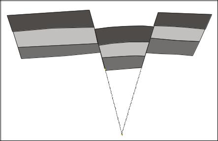
When the reservoir grid has been finalised in advance, this embedding is normally done by adding grid blocks to all sides of the reservoir, typically extending grid block directions and with increasing block sizes towards the edges, a task that can be done with dedicated software. (For an Eclipse – Visage coupling the embedding can be done in the Visage suite program VisGen.) Although some constraints can be put on the grid extension process, the embedding is normally carried out without any attempt to honour actual rock topology in the extension area. A typical embedding of a simple reservoir grid is shown in Figure A1, where the original reservoir grid is shown as the thin blue slab in the middle of the final grid.

Figure A1. Embedding of Reservoir Grid

Since few if any reservoir engineers have such an embedding in mind when building the reservoir grid, the extension process can frequently run into problems. The commonly occurring problems are tied to non-consistent grids as discussed above, and the use of non-vertical coordinate lines, which will be discussed here.

110

Non-vertical coordinate lines

Coordinate lines can have any (non-horizontal) direction, and non-vertical coordinate lines are primarily used to honour actual fault geometries. Figure A2 shows a cross section of a fault block which bounding faults sloping in different directions.

Figure A2. Coordinate lines and sloping faults (cross section view)

The coordinate lines A and B pose no problems in the reservoir grid (indicated by shades of grey). But if an underburden is added below the grid, lines A and B will intersect somewhere below the reservoir. Since the thickness of the over / underburden is normally several reservoir thicknesses, this problem is almost certain to emerge in the embedding process whenever not all coordinate lines are parallel.

Fixing the problems at this stage is not a trivial task – especially if non-consistencies have to be fixed at the same time.

Hence the obvious recommendation is, for grids which are to be used in coupled simulations, to build the entire grid including the embedding with the final purpose in mind from the outset. This will often enforce compromises between desires / requirements for the reservoir grid and the embedded grid, but such conflicts are better solved when regarding all aspects of the problem simultaneously. (Certainly this advice is not easily applied to existing grids which have taken a considerable time to build, and where a request to redo the job is not welcomed…)

As an example, the situation depicted in Figure A2 cannot be resolved accurately. The intersecting coordinate lines cannot be accepted, so an adjustment of the fault slopes such that the coordinate lines A and B only just don’t intersect in the underburden is perhaps to live with.

Honouring material properties of non-reservoir rock.

Aquifers

Aquifers should be handled differently in a coupled model than in flow simulation. Analytic or numeric aquifers are a convenient means of simulating aquifer pressure support to the reservoir, but cannot been used in such a setting when including rock mechanics effects. The aquifer is also a volume of porous soil, and hence it influences directly both the stress state and the reservoir pressure. Aquifers are a prime example of why we encourage to build the grid with the final embedded model as goal from the outset, not as a two-stage process.

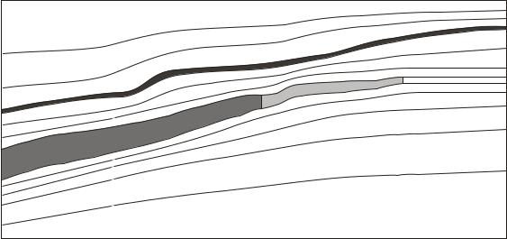
Figure A3 is an example where the reservoir is connected to a large aquifer extending into the sideburden. This volume should obviously be modelled as fluid-bearing porous rock, not as soil inactive to flow as would result from a build-on embedding process. Note that a traditional numerical aquifer would not work here, since there is no way the node displacements in the aquifer volume could be accurately computed or accounted for by such an approach.

111