p41

The scale plays here a similar role to the renormalization scale introduced in the second lecture. Its choice is arbitrary, and f (x; Q2) should not depend on it. Requiring this independence, we get the following “renormalization-group invariance” condition:

This equation is usually called the DGLAP (Dokshitzer-Gribov-Lipatov-Altarelli-Parisi) equation. As in the case of the resummation of leading logarithms in Re+e induced by the RG invariance constraints,

the DGLAP equation – which is the result of RG-invariance – resums a full tower of leading logarithms of Q2.

The first derivative is given by the DGLAP equation itself. Higher derivatives can be obtained by differentiating it:

The n-th term in this expansion, proportional to ( s t)n, corresponds to the emission of n gluons (it is just the n-fold iteration of what we did studying the one-gluon emission case).

With similar calculations one can include the effect of the other O( s) correction, originating from the splitting into a qq pair of a gluon contained in the proton. With the addition of this term, the evolution equation for the density of the ith quark flavour becomes:

In the case of interactions with a coloured probe (say a gluon) we meet the following corrections, which

71

it is easy to prove that the evolution equations turn into ordinary linear differential equations:

5.3.Properties of the evolution equations

We now study some general properties of these equations. It is convenient to introduce the concepts of valence (V (x; t)) and singlet ( (x; t)) densities:

i{

XX

where the index { refers to the antiquark flavours. The evolution equations then become:

Note that the equation for the valence density decouples from the evolution of the gluon and singlet densities, which are coupled among themselves. This is physically very reasonable, since in perturbation theory the contribution to the quark and the antiquark densities coming form the evolution of gluons (via their splitting into qq pairs) is the same, and will cancel out in the definition of the valence. The valence therefore only evolves because of gluon emission. On the contrary, gluons and qq pairs in the proton sea evolve into one another.

72

Since V (1) itself in different from 0, we obtain a constraint on the first moment of the splitting function:

= 0. This constraint is satisfied by including the effect of the virtual corrections, which generate

Another sum rule which does not depend on Q2 is the momentum sum rule, which imposes the constraint that all of the momentum of the proton is carried by its constituents (valence plus sea plus gluons):

Once more this relation should hold for all Q2 values, and you can prove by using the evolution equations that this implies:

You can check using the definition of second moment, and the explicit expressions of the Pqq and Pgq splitting functions, that the first condition is automatically satisfied. The second condition is satisfied by including the virtual effects in the gluon propagator, which contribute a term proportional to (1 z). It is a simple exercise to verify that the final form of the Pgg (z) splitting function, satisfying Eq. (180), is:

5.4.Solution of the evolution equations

The evolution equations formulated in the previous section can be solved analytically in moment space. The boundary conditions are given by the moments of the parton densities at a given scale , where in principle they can be obtained from a direct measurement. The solution at different values of the scale Q can then be obtained by inverting numerically the expression for the moments back to x space. The resulting evolved densities can then be used to calculate cross sections for an arbitrary process involving hadrons, at an arbitrary scale Q. We shall limit ourselves here to studying some properties of the analytic solutions, and will present and comment some plots obtained from numerical studies available in the literature.

As an exercise, you can show that the solution of the evolution equation for the valence density is the following:

where the running of s( 2) has to be taken into account to get the right result. Since all moments P (n) are negative, the evolution to larger values of Q makes the valence distribution softer and softer. This is physically reasonable, since the only thing that the valence quarks can do is to loose energy because of gluon emission.

73

Fig. 2: Left:Valence up-quark momentum-density distribution, for different scales Q. Right: gluon momentum-density distri-

bution.

The solutions for the gluon and singlet distributions fg and can be obtained by diagonalizing the 2 2 system in Eqs. (174) and (175). We study the case of the second moments, which correspond to the momentum fractions carried by quarks and gluons separately. In the asymptotic limit (2) goes to a constant, and = 0. Then, using the momentum sum rule:

As a result, the fraction of momentum carried by gluons is asymptotically approximately 50% of the total proton momentum. It is interesting to note that, experimentally, this asymptotic value is actually reached already at rather low values of Q2. It was indeed observed already since the early days of the DIS experiments that only approximately 50% of the proton momentum was carried by charged constituents. This was one of the early evidences for the existence of gluons.

As I mentioned earlier, a complete solution for the evolved parton densities in x space can only be obtained from a numerical analysis. This work has been done in the past by several groups (see e.g. the discussions in Ref. [8]), and is continuously being updated by including the most up-to-date experimental results used for the determination of the input densities at a fixed scale. Figure 2a describes the up-quark valence momentum density at different scales Q. Note the anticipated softening at large scales, and the clear logQ2 evolution. The most likely momentum fraction carried by a valence up quark in the proton goes from x 20% at Q = 3 GeV, to x < 10% at Q = 1000 GeV. Notice finally that the density vanishes at small x.

Figure 2b shows instead the gluon momentum density at different scales Q. This time the density grows at small-x, with an approximate g(x) 1=x1+ behaviour, and > 0 slowly increasing at large Q2. This low-x growth is due to the 1=x emission probability for the radiation of gluons, which was discussed in the previous lecture and which is represented by the 1=x factors in the Pgq(x) and

74

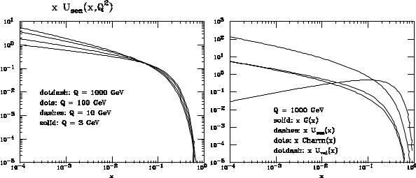
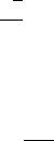
Fig. 3: Left: Sea up-quark momentum-density distribution, for different scales Q. Right: Momentum-density distribution for

several parton species, at Q = 1000 GeV.

Pgg (x) splitting functions. Figure 3a shows the up-quark sea momentum density at different scales Q. Shape and evolution match those of the gluon density, a consequence of the fact that sea quarks come from the splitting of gluons. Since the gluon-splitting probability is proportional to s, the approximate ratio sea=gluon 0:1 which can be obtained by comparing Figs. 2b and 3a is perfectly justified.

Finally, the momentum densities for gluons, up-sea, charm and up-valence distributions are shown in Fig. 3b for Q = 1000 GeV. Note here that usea and charm are approximately the same at very large Q and small x, The proton momentum is mostly carried by valence quarks and by gluons. The contribution of sea quarks is negligible.

6.QCD IN HADRONIC COLLISIONS

In hadronic collisions, all phenomena are QCD-related. The dynamics is more complex than in e+e or DIS, since both beam and target have a non-trivial partonic structure. As a result, calculations (and experimental analyses) are more complicated. QCD phenomenology is however much richer, and the higher energies available in hadronic collisions allow to probe the structure of the proton and of its constituents at the smallest scales attainable in a laboratory.

Contrary to the case of e+e and lepton-hadron collisions, where calculations are routinely available up to next-to-next-to-leading order (NNLO) accuracy, theoretical calculations for hadronic collisions are available at best with next-to-leading-order (NLO) accuracy. The only exception is the case of Drell-Yan production, where NNLO results are known for the total cross sections. So we generally have relatively small precision in the theoretical predictions, and theoretical uncertainties which are large when compared to LEP or HERA.

However, pp collider physics is primarily discovery physics, rather than precision physics (there are exceptions, such as the measurements of the W mass and of the properties of b-hadrons. But these are not QCD-related measurements). As such, knowledge of QCD is essential both for the estimate of the expected signals, and for the evaluation of the backgrounds. Tests of QCD in pp collisions confirm our understanding of perturbation theory, or, when they fail, point to areas where our approximations need to be improved. (see, e.g., the theory advances prompted by the measurements of production at CDF!).

75

Finally, a reliable theoretical control over the details of production dynamics allows one to extract important information on the structure of the proton (parton densities) in regions of Q2 and x otherwise unaccessible. Control of QCD at the current machines (the Tevatron at Fermilab) is therefore essential for the extrapolation of predictions to higher energies (say for applications at the future LHC, at CERN).

The key ingredients for the calculation of production rates and distributions in hadronic collisions are:

the matrix elements for the hard, partonic process (e.g., 0 ,

gg ! gg; gg ! bb; qq ! W; : : :)

the hadronic parton densities, discussed in the previous lecture.

Then the production rate for a given final state H is given by a factorization formula similar to the one used to describe DIS:

where the parton densities fi's are evaluated at a scale Q typical of the hard process under consideration. For example Q ' MDY for production of a Drell-Yan pair, Q ' ET for high transverse-energy (ET ) jets, Q2 ' p2T + m2Q for high-pT heavy quarks, etc.

In this lecture we will briefly explore two of the QCD phenomena currently studied in hadronic collisions: Drell-Yan, and inclusive jet production. More details can be found in Refs. [8,4].

6.1.Drell-Yan processes

While the Z boson has been recently studied with great precision by the LEP experiments, it was actually discovered, together with the W boson, by the CERN experiments UA1 and UA2 in pp collisions. W physics is now being studied in great detail at LEP2, but the best direct measurements of its mass by a single group still belong to pp experiments (CDF and D0 at the Tevatron). Even after the ultimate luminosity will have been accumulated at LEP2, with a great improvement in the determination of the parameters of the W boson, the monopoly of W studies will immediately return to hadron colliders, with the Tevatron data-taking resuming in the year 2000, and later on with the start of the LHC experiments.

Precision measurements of W production in hadronic collisions are important for several reasons:

this is the only process in hadronic collisions which is known to NNLO accuracy

the rapidity distribution of the charged leptons from W decays is sensitive to the ratio of the up and down quark densities, and can contribute to our understanding of the proton structure.

deviations from the expected production rates of highly virtual W 's (pp ! W ! e ) are a possible signal of the existence of new W bosons, and therefore of new gauge interactions.

The partonic cross-section for the production of a W boson from the annihilation of a qq pair can be easily calculated, giving the following result [8,4]:

where s^ is partonic center of mass energy squared, and Vij is the element of the Cabibbo-Kobayashi- Maskawa matrix. The delta function comes from the 2 ! 1 phase space, which forces the center-of-mass energy of the initial state to coincide with the W mass. It is useful to introduce the two variables

76

where Shad is the hadronic center of mass energy squared. The variable y is called rapidity. For slowly moving objects it reduces to the standard velocity, but, contrary to the velocity, it transforms additively even at high energies under Lorentz boosts along the direction of motion. Written in terms of and y, the integration measure over the initial-state parton momenta becomes: dx1dx2 = d dy. Using this expression and Eq. (188) in Eq. (187), we obtain the following result for the LO total W production cross

where the function ij is usually called partonic luminosity. In the case of collisions, the overall

L ( ) ud

factor in front of this expression has a value of approximately 6.5 nb. It is interesting to study the partonic luminosity as a function of the hadronic CoM energy. This can be done by taking a simple approximation

for the parton densities. Following the indications of the figures presented in the previous lecture, we shall assume that fi(x) 1=x1+ , with < 1. Then

The DY cross-section grows therefore at least logarithmically with the hadronic CM energy. This is to be compared with the behaviour of the Z production cross section in e+e collisions, which is steeply diminuishing for values of s well above the production threshold. The reason for the different behaviour in hadronic collisions is that while the energy of the hadronic initial state grows, it will always be possible to find partons inside the hadrons with the appropriate energy to produce the W directly on-shell. The number of partons available for the production of a W is furthermore increasing with the increase in hadronic energy, since the larger the hadron energy, the smaller will be the value of hadron momentum fraction x necessary to produce the W . The increasing number of partons available at smaller and smaller values of x causes then the growth of the total W production cross section.

A comparison between the best available prediction for the production rates of W and Z bosons in hadronic collisions, and the experimental data, is shown in Fig. 4. The experimental uncertainties will soon be dominated by the limited knowledge of the machine luminosity, and will exceed the accuracy of the NNLO predictions. This suggests that in the future the total rate of produced W bosons could be used as an accurate luminometer.

It is also interesting to note that an accurate measurement of the relative W and Z production rates (which is not affected by the knowledge of the total integrated luminosity, that will cancel in their ratio) provides a tool to measure the total W width. This can be seen from the following equation:

As of today, this technique provides the best measurement of W : W = 2:06 0:06 GeV, which is a factor of 5 more accurate than the current best direct measurements from LEP2.

77

Center of Mass Energy (TeV)

Fig. 4: Comparison of measured (a) B(W ! e ) and (b) B(Z0 ! e+e ) to 2-loop theoretical predictions using MRSA parton distribution functions. The UA1 and UA2 measurements and D0 measurements are offset horizontally by 0.02 TeV for clarity. In the inset, the shaded area shows the 1 region of the CDF measurement; the stars show the predictions using various parton distribution function sets (1) MRSA, (2) MRSD00, (3)MRSD-0, (4) MRSH and (5) CTEQ2M. The theoretical points include a common uncertainty in the predictions from choice of renormalization scale (MW =2 to 2MW ).

6.2.W rapidity asymmetry

The measurement of the charge asymmetry in the rapidity distribution of W bosons produced in pp collisions can provide an important measurement of the ratio of the u-quark and d-quark momentum distributions. Using the formulas provided above, you can in fact easily check as an exercise that:

We can then construct the following charge asymmetry (assuming the dominance of the quark densities over the antiquark ones, which is valid in the kinematical region of interest for W production at the Tevatron):

78

Setting fd(x) = fu(x) R(x) we then get:

p exp( y)4. The current CDF data provide the most accurate measurement to date of this quantity (see Ref. [8]).

6.3.Jet production

Jet production is the hard process withpthe largest rate in hadronic collisions. For example, the cross section for producing at the Tevatron ( Shad = 1:8 TeV) jets of transverse energy ETjet < 50 GeV is of the order of a b. This means 50 events/sec at the luminosities available at the Tevatron. The data collected at the Tevatron so far extend all the way up to the ET values of the order of 450 GeV. These events are generated by collisions among partons which carry over 50% of the available pp energy, and allow to probe the shortest distances ever reached. The leading mechanisms for jet production are shown in Fig. 5.

Fig. 5: Representative diagrams for the production of jet pairs in hadronic collisions.

The 2-jet inclusive cross section can be obtained from the formula

that has to be expressed in terms of the rapidity and transverse momentum of the quarks (or jets), in order to make contact with physical reality. The two-particle phase space is given by

where kT is the transverse momentum of the final-state partons. Here y is the rapidity of the produced

4In practice one cannot determine x1;2 with arbitrary precision on an event-by-event basis, since the longitudinal momentum of the neutrino cannot be easily measured. The actual measurement is therefore done by studying the charge asymmetry in the rapidity distribution of the charged lepton.

79

parton in the parton CM frame. It is given by

where y1 and y2 are the rapidities of the produced partons in the laboratory frame (in fact, in any frame). One also introduces

with being usually referred to as pseudorapidity.

The leading-order Born cross sections for parton parton scattering are reported in Table 1. It is interesting to note that a good approximation to the exact results can be easily obtained by using the softgluon techniques introduced in the third lecture. Based on the fact that even at 90 min(jtj; juj) does not exceed s=2, and that therefore everything else being equal a propagator in the t or u channel contributes to the square of an amplitude 4 times more than a propagator in the s channel, it is reasonable to assume that the amplitudes are dominated by the diagrams with a gluon exchanged in the t (or u) channel. It is easy to calculate the amplitudes in this limit using the soft-gluon approximation. For example, the

80