Biblio5

604 REVIEW OF MATHEMATICS FOR TELECOMMUNICATION APPLICATIONS

Table B.2 Selected Numbers and their Logarithms

log−1 1.3010 c 19.9986.

Enter the number in the calculator so it appears on the display. Press 2nd or “shift.” Press the “log” button. Now 19.9986 appears on the display. The particular calculator we are using indicates that this is the 10x function, which uses the same button as the “log” function, but on the “shift” or second level of the calculator.

There are a number of mathematical calculations that are either very difficult to do without the application of logarithms, or nearly impossible. One such operation is to calculate the cube root (or 4th, 5th to the nth root).

Example. Calculate the cube root of 9751.

Enter 9751 in the calculator and press the “log” button to get the logarithm of the number. Divide the logarithm by 3 and get the antilog of the result.

B.5 ESSENTIALS OF TRIGONOMETRY

B.5.1 Definitions of Trigonometric Functions

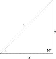
Figure B.1 is a right triangle. Remember that a right triangle has one angle that is 908 by definition.

The basic trigonometric functions are defined as follows:

The following are some initial trigonometric relationships:

The triangle in Figure B.1 has a 908 angle and two acute angles. We denominated one of the acute angles v. Now let us call those two acute angles, A and B. First rule: angle A + angle B + 908 1808. In fact, this rule will hold for any triangle; it does not necessarily have to be a rightc triangle.

The following are useful relationships for a right triangle with acute angles A and B:

x 2/ r 2 + y 2/ r 2 c 1.

From the basic trigonometric functions we can substitute:

606 REVIEW OF MATHEMATICS FOR TELECOMMUNICATION APPLICATIONS

sin2 v + cos2 v c 1.

If both terms on the left-hand side of the preceding equation are divided by cos2 v, we then have:

1 + tan2 v c sec2 v.

In a similar manner, if we divide the two left-hand terms by sin2 v, we have:

1 + cot2 v c csc2 v.

The preceding relationships are called fundamental trigonometric identities.

There are three common acute angles that are used repeatedly in geometry and trigonometry. These are 308, 458, and 608. If we know any one of these angles in a right triangle, the other angles are also known. Remember the sum of the three angles is 1808. Of course, with a scientific calculator, the trigonometric functions are easy to obtain. With many scientific calculators, there will be only buttons for three trigonometric functions: sin, cos, and tan. Using the relationships previously provided, sec, csc, and cot can be simply calculated using the inverse key (1/ X button).

The following are some algebraic exercises using trigonometric functions. Sometimes

B.5.2 Trigonometric Function Values for Angles Greater than 908

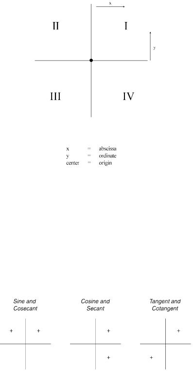
The standard graph based on rectangular coordinates is broken up into four quadrants around the origin, as illustrated in Figure B.2. Some of the trigonometric function values will be negative for angles greater than 908. Guidance for the assignment of either positive or negative values may be found in Figure B.3. Here only positive values are shown. For all other quadrants, negative values must be assigned.

Most scientific calculators will assign the proper sign for angles greater than 908. Most trig function tables and older scientific calculators required that the angle be ≤ 908. When such a situation arises, we subtract the angle from either 1808 or 3608, and we assign the proper sign based on Figure B.3.

Examples and Discussion. Obtain values of the indicated trigonometric functions and angles.

Figure B.2 A typical graph for plotting with rectangular coordinates showing the four quadrants.

cos1208 c −0.5 or cos(180 − 1208) c cos608 c 0.5. Apply proper sign from Figure B.3 or cos1208 c −0.5.

tan2008 c 0.3640 or tan(200 − 1808) c tan208 c 0.3640; the sign is positive from Figure B.3.

Given the Trigonometric Function Value, Find the Equivalent Angle. Find the value for v for the following:

Figure B.3 Quadrant sign diagram. Only positive signs are shown. All other quadrants require negative values.

608 REVIEW OF MATHEMATICS FOR TELECOMMUNICATION APPLICATIONS

sin v c 0.2952.

Enter 0.2952 in the calculator display, press 2nd or “shift” and then the sin key, and we get 17.178. On many calculators, just above the sin button or key one will find sin−1. This means that given the sin of the angle, find the angle. The reader should realize there is also a valid value in the second quadrant, namely, 180 − 17.178 c 162.838.

cos v c −0.8654.

Enter 0.8654 on the calculator display. Press 2nd or “shift” and then depress the cos key or−button. We get v c 149.938.

tan v c 1.6055. Find the third quadrant value (see Figure B.3).

v c 58.088 in the first quadrant, 180 + 58.088 c 238.088, in the third quadrant. Appendix B is based on the author’s experience and Refs. 1, 2, and 3.

REFERENCES

1. G. James and R. C. James, Mathematics Dictionary, 3rd ed., D. Van Nostrand & Co., Princeton, NJ, 1968.

2. W. R. Van Voorhis and E. E. Haskins, Basic Mathematics for Engineers and Science, PrenticeHall, Englewood Cliffs, NJ, 1952.

3. L. A. Kline and J. Clark, Explorations in College Algebra, Wiley, New York, 1998.

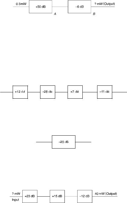
We now have learned how to handle power ratios of 10, 100, 1000, and so on, and 0.1, 0.01, 0.001, and so on. These, of course, lead to dB values of +10 dB, +20 dB, and +30 dB; −10 dB, −20 dB, −30 dB, and so on. The next step we will take is to learn to derive dB values for power ratios that lie in between 1 and 10, 10 and 100, 0.1 and 0.01, and so on.

One excellent recourse is the scientific calculator. Here we apply a formula (C1.1). For example, let us deal with the following situation:

Because the output of this network is greater than the input, the network has a gain. Keep in mind we are in the power domain; we are dealing with mW. Thus:

dB value c 10 log 4/ 2 c 10 log 2 c 10 × 0.3010 c +3.01 dB.

We usually round-off this dB value to +3 dB. If we were to do this on our scientific calculator, we enter 2 and press the log button. The value 0.3010– – – appears on the display. We then multiply (× ) this value by 10, arriving at the +3.010 dB value.

This relationship should be memorized. The amplifying network has a 3-dB gain because the output power was double the input power (i.e., the output is twice as great as the input).

For the immediately following discussion, we are going to show that under many situations a scientific calculator is not needed and one can carry out these calculations in his or her head. We learned the 3-dB rule. We learned the +10, +20, +30 dB; −10, −20, −30 (etc.) rules. One should be aware that with the 3-dB rule, there is a small error that occurs two places to the right of the decimal point. It is so small that it is hard to measure.

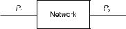
With the 3-dB rule, multiples of 3 are easy. If we have power ratios of 2, 4, and 8, we know that the equivalent (approximate) dB values are +3 dB, +6 dB, and +9 dB, respectively. Let us take the +9 dB as an example problem. A network has an input of 6 mW and a gain of +9 dB. What power level in mW would we expect to measure at the output port?

One thing that is convenient about dBs is that when we have networks in series, each with a loss or gain given in dB, we can simply sum the values algebraically. Likewise, we can do the converse: We can break down a network into hypothetical networks in series, so long as the algebraic sum in dB of the gain/ loss of each network making up the whole is the same as that of the original network. We have a good example with the preceding network displaying a gain of +9-dB. Obviously 3 × 3 c 9. We break down the +9-dB network into three networks in series, each with a gain of +3 dB. This is shown in the following diagram:

612 LEARNING DECIBELS AND THEIR APPLICATIONS

We should be able to do this now by inspection. Remember that +3 dB is double the power; the power at the output of a network with +3-dB gain has 2× the power level at the input. Obviously the output of the first network is 12 mW (point A above). The input to the second network is now 12 mW and this network again doubles the power. The power level at point B, the output of the second network, is 24 mW. The third network—double the power still again. The power level at point C is 48mW.

Thus we see that a network with an input of 6 mW and a 9-dB gain, will have an output of 48 mW. It multiplied the input by 8 times (8 × 6 c 48). That is what a 9-dB gain does. Let us remember: +3 dB is a two-times multiplier; +6 dB is a four-times multiplier, and +9 dB is an eight-times multiplier.

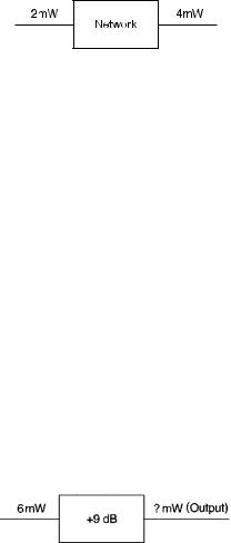
Let us carry this thinking one step still further. We now know how to handle 3 dB, whether + or −, and 10 dB (+ or −), and all the multiples of 10 such as 100,000 and 0.000001. Here is a simple network. Let us see what we can do with it.

We can break this down into two networks using dB values that are familiar to us:

If we algebraically sum the +10 dB and the −3 dB of the two networks in series shown above, the result is +7 dB, which is the gain of the network in question. We have just restated it another way. Let us see what we have here. The first network multiplies its input by 10 times (+10 dB). The result is 15 × 10 or 150 mW. This is the value of the level at A. The second network has a 3-dB loss, which drops its input level in half. The input is 150 mW and the output of the second network is 150 × 0.5, or 75 mW.

This thinking can be applied to nearly all dB values except those ending with a 2, 5, or 8. Even these values can be computed without a calculator, but with some increase in error. We encourage the use of a scientific calculator, which can provide much more accurate results, from 5 to 8 decimal places.

Consider the following problem: