

An_Airborne_X-band_Synthetic_Aperture_Radar
.pdf1.5. OVERVIEW OF THE THESIS |
CHAPTER 1. INTRODUCTION |
•The transceiver shall have switchable gain i.e. both manual and automatic gain.
•Sensitivity Time Control (STC) capability should be implemented in the system.
•The system shall be built with extensive Built-in Test (BIT) capabilities to allow for preflight testing in the laboratory.
•The system shall be designed with default operating mode i.e. function in the receiver mode and not in BIT mode.
1.5Overview of the Thesis
The dissertation starts with an overview of synthetic aperture radar in Chapter 2. In this chapter, the theory that is used to design the system is explained. The derivations of the terms and formulas used in the following chapters are presented here. Section 2.2 describes the pulsed radar concept with an explanation of the radar equation. The centre frequency used is important in choosing the size of the antenna and the depth of radar penetration required in this project. The beamwidth relates to the swath width, antenna gain and hence antenna size. Section 2.3 introduces the SAR concepts, vital in designing the receiver, with reference to the geometry of the airborne radar configuration. Azimuth compression in SAR, is used to boost the signal power of a point-like target over noise. Finally, an explanation of the relationship between the PRF and doppler bandwidth is provided.
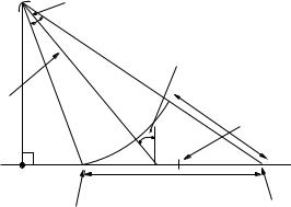
In Chapter 3 the front-end power return of SASAR II radar is discussed. The terms and theory developed in Chapter 2 are used in the radar equation. Two types of targets are considered namely point targets and distributed targets. The corner reflector at RRSGUCT is used to estimate the power return of large point-like targets. Figure 1.1 shows the mainbeam setup of the antenna pointing to the Earth with the boresight axis closer to the near-swath. Two gain pattern simulations have also been investigated namely cosecantsquared and sinc-squared antenna pattern as explained in Section 3.4. The latter proved to be the more appropriate one in providing the highest gain. Section 3.5 describes the distributed targets used in the design, such as trees and wheat fields and are chosen from models described by Ulaby [15]. Point-like targets are also expected to be present in the swath width and their radar cross section are calculated in Section 3.5.3. The backscattered power is simulated at the front-end of the antenna as described in Section 3.6 for varying terrain types and point targets that the radar might encounter. The design also includes the different scenarios with the boresight axis of the antenna at near-swath, midswath and far-swath. The incidence angle used for near-swath is set to 40◦ relating to a
3
1.5. OVERVIEW OF THE THESIS |
CHAPTER 1. INTRODUCTION |
φ e , Elevation Beamwidth
|
Incidence Angle, θ |
|
|
i |
|
Boresight axis |
slant range |
|
swath width |
||
|
Mid−swath
Nadir Point
Ground Range Swath Width
Near−swath |
Far−swath |
Figure 1.1: Side Geometry with the 3-dB Beamwidth Covering the Swath Width.
maximum ground range of 11513 m for 8192 range bins. The bandwidth of the system used in simulation for the front-end was set to 200 MHz and tailored to reach 100 MHz as explained in Chapter 4.
The receiver is broken down into 2 intermediate frequencies (IFs) stages and a radio frequency (RF) stage as shown in Figure 1.2. The particular IFs were chosen to match those frequencies of previous projects such that future expansion of the system could be performed. Chapter 4 describes the RF and IF stages of the receiver. The use of a dual conversion receiver is required to relieve the streneous cut-off required for the RF filter in order to attenuate the image frequency response to a minimum. A justification of the different components used is laid out in this chapter and the transfer function of the system is worked out. The theory and properties associated with the components are investigated. The low noise amplifier (LNA) is used in the front end of the system to set the noise figure of the receiver as is described in Sections 4.2 and 4.4. Simulations are done with varying gains so as not to saturate the components in the later stages of the receiver and a maximum gain of 22 dB is selected. The use of the image rejection filter in the RF stage is explained in Section 4.5. Section 4.6 deals with mixers, conversion loss and intermodulation distortions. The relative output of the 2 mixers, which consists of the RF and spurious responses, are displayed. Section 4.7 shows plots of the transfer function of the IF filters used in rejecting out-of-band signals.
A sensitivity time control (STC) is implemented using an electronic attenuator and gain blocks as explained in Section 4.8. To prevent the receiver from being overloaded by strong echoes from nearby terrains, objects and targets, the STC is used to lower the gain for the early part of the interpulse period and gradually increases the gain for the return from the far range. This in effect causes the return power to be fairly constant over the interpulse period. From simulations performed in Chapter 3, an attenuator of 20 dB
4

1.5. OVERVIEW OF THE THESIS |
CHAPTER 1. INTRODUCTION |
TRANSMITTER |
DUPLEXER |
T |
|
R |
|||
|
|
||
|
Antenna |
|
|
|
Antenna Output |
||
RF STAGE |
rd |
IF |
|
@ 9300MHz |
3 |
||
|
|
||
IF STAGE |
nd |
|
|
2 |
IF |
||
@ 1300MHz |
|||
|
|
SENSITIVITY TIME CONTROL
1st IF @ 158 MHz
MANUAL
GAIN
CONTROL
TO ADC
RECEIVER
Figure 1.2: Receiver Block Diagram
dynamic range should suffice.
The MGC is a user-switchable gain. The implementation using a digital attenuator is also described in Section 4.8. Its main function is to switch the gain to different user-defined values depending on the terrain being imaged. From the receiver level tables of Section 4.11 and simulations of maximum return signal and noise level, an attenuation of dynamic range of 30 dB is required.
The receiver-power-level table and the receiver-power-level diagram are two important tools in designing and implementing a receiver such that no components are driven into saturation thereby generating harmonics. With an 8-bit analogue-to-digital converter (ADC) of peak voltage of 1 V, the maximum instantaneous power input is 13 dBm. The maximum power return from large targets, as modelled in Chapter 3, is -55.3 dBm and hence, a 60 dB gain receiver is designed to boost the signal input up to a maximum of 7 dBm. For an antenna facing a blackbody, which is the Earth for this project, the noise temperature is 290 K . The thermal noise is thus calculated at the antenna output and is tracked down the receiver together with noise generated by the different components like the LNA, mixers, IF amplifiers and attenuators. The theoretical receiver noise temperature is worked out to be a minimum of 222 K from the available specifications of the individual components with attenuation being at its minimum.
5
1.5. OVERVIEW OF THE THESIS |
CHAPTER 1. INTRODUCTION |
The largest power return and noise level at the front-end of the receiver predicts a dynamic range of 40 dB. Amplification is required to boost the signal but at the same time noise generated by the system has to be taken into account and ways of limiting this noise are discussed. The mixers, filters and amplifiers used are justified in this chapter. Intermodulation products are investigated together with the effects of image frequency contribution in undermining the system.
Chapter 5 lays out the different tests that are performed on the IFs of the receiver. The tests are performed on each of the 4 sections namely,
1.3rd IF (RF stage or 3rd IF)
2.2nd IF (L-band stage or 2nd IF)
3.1st IF (1st IF STC)
4.1st IF (1st IF MGC)
The gain, insertion loss tests are performed on each stage individually and the output spectrum is mesaured for different frequency of interest. The insertion loss tests basically ascertain that no components are driven into saturation. A signal is injected, at a power level designed in the receiver-level table for minimum MGC attenuation, in each of the four sections and the output is measured and compared with the expected output. Varying the frequency of the input signal helps in testing the cut-off of the filters in the different sections.
Noise figure tests are performed on the system as a whole for minimum and maximum attenuation of the MGC attenuator in Section 5.7 and the output power level of the signal at band centre versus signal on either side is measured in Section 5.8.
Chapter 6 gives the conclusions and recommendations for future work on the receiver based on the design and tests performed. The receiver works according to the design. The simulated power return for a corner reflector is −55.3 dBm. The components are not driven into saturation when a signal of −50 dBm is injected at the front-end of the receiver. The cascaded filters result in a 3-dB bandwidth of 94 MHz at the ADC input.
6
Chapter 2
Theory of Airborne SAR
2.1 Introduction
The theory underlying the development of the Airborne SASAR II system is explained in this chapter. The analysis of the terms used in the design of the radar receiver is presented, as they appear in the radar equation, which remains fundamental to radar design. Section 2.2 introduces the concept related to pulse radar with the properties of a radar that affect transmission of a pulse. Section 2.3 lays out the basics of SAR, with an explanation of the parameters crucial to the radar receiver design. An important characteristic of a SAR image is its resolution, which is defined in terms of minimum distance at which two closely spaced scatterers of equal strength may be resolved. SAR and conventional radar achieve slant range resolution in a similar way by using pulse-ranging technique. However, SAR is distinctive in achieving along-track (azimuth) resolution by using aperture synthesis and is defined in terms of the antenna dimension only.
2.2 Pulsed Radar Basics
The detection range of a radar system is primarily a function of three variables, namely:
1.Transmitted Power.
2.Antenna Gain.
3.Receiver Sensitivity.
An increase in transmitted power will increase the amount of energy radiated and hence, the backscattered power from the target will be stronger. The antenna gain is a measure of
7
2.2. PULSED RADAR BASICS |
CHAPTER 2. THEORY OF AIRBORNE SAR |
the radiated energy towards the target as opposed to uniform radiation of energy. Receiver sensitivity is a measure of the capability of the receiver in detecting target returns.
2.2.1 Antenna Gain
Antenna gain describes the degree to which an antenna concentrates electromagnetic energy in a narrow angular beam. The two parameters associated with the gain of an antenna are the directive gain and directivity. The gain of an antenna serves as a figure of merit relative to an isotropic source with the directivity of an isotropic antenna being equal to 1 by definition [14].
The directive gain, G, of an antenna at a far-field distance, R, is defined as the ratio [7, pg6.3],
G = |
maximum radiation intensity |
|
|
average radiation intensity |
|
= |
maximum power per steradian |
|
|
total power radiated/4π |
|
The far-field region is assumed in this project unless otherwise stated and is the region defined by the inequality [14, pg72],
|
|
|
R ≥ |
2d2 |
|
|
(2.1) |
|||
|
|
|
|
λ |
|
|
|
|
||
where d is the antenna aperture length. |
|
|
|
|||||||
This ratio can also be expressed in terms of maximum radiated power density |
|
W |
at a |
|||||||
|
2 |
|||||||||
|
R |
|
|
|
|
|
|
|
m |
|
far-field distance, |
|
, over the power density radiated by an isotropic source at |
! |
|
" |
|||||
distance, |
|
|
|
|
|
|
|
|
|
|
|
|
G = |
maximum power density |
|
|
|
||||
|
|
total power radiated/4πR2 |
|
|
|
|
||||
|
|
= |
pmax |
|
|
(2.2) |
||||
|
|
Prad/4πR2 |
|
|
|
|||||
Equation 2.2 shows how much stronger the actual maximum power density is, than it would be if the radiated power was distributed isotropically.
The directivity, Dmax, is defined as the value of the directive gain in the direction of its maximum value [14, pg77].
The gain of an antenna is related to the directivity is given by,
8
2.2. PULSED RADAR BASICS |
CHAPTER 2. THEORY OF AIRBORNE SAR |
G = ϵ Dmax |
(2.3) |
The radiation efficiency, ϵ, is given by,
ϵ = |
Prad |
= |
Ptx |
(2.4) |
|
Ptx + Ploss |
|||
|
Ptx |
|
||
where Ptx is the power coupled into the antenna and Prad being the actual power being radiated.
2.2.2 Antenna Radiation Pattern
The gain of an antenna also varies with the type of antenna pattern as explained in [10, pg29]. It relates the distribution of electromagnetic energy in angular space. For a pencil beam antenna with a sinc-squared pattern, the normalized power radiation pattern in azimuth direction, φ, is given by,
|
|
# |
$! |
πd |
" |
% |
& |
2 |
|
|
2 |
sin |
|
sin(η) |
|
(2.5) |
|||
|E(φ)| |
= |
! |
πλd |
sin(η) |
|
||||
|
|
|
|
" |
|
|
|
|
|
where η is the angle off boresight.
The directive gain of an antenna can also be expressed in terms of its physical dimension. The aperture of an antenna is equal to its physical area projected on a plane orthogonal to the direction of the mainbeam. The directive gain is given in [7] by,
G = |
4πAe |
|
(2.6) |
|
λ2 |
||||
|
|
|||
where Ae is the effective aperture. |
|
|
|
|
The derivation of Equation 2.6 to calculate antenna gain is explained in [6, |
pg9]. The |
|||
3-dB (half-power) beamwidth of an antenna with aperture size, d, is given in [10] by,
|
|
|
|
φ = |
0.88λ |
(2.7) |
|||
|
|
|
|
|
|
|
|||
|
|
|
|
|
d |
||||
|
|
|
|
|
|
|
|||
|
|
|
|
|
λ |
|
|||
|
|
|
|
≈ |
|
[radians] |
(2.8) |
||
|
|
|
|
d |
|||||
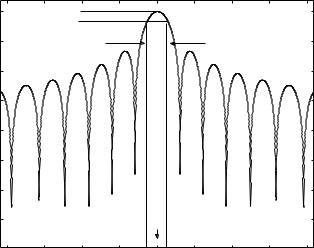
Figure 2.1 shows the “ |
|
sin(x) |
2 |
” antenna pattern for a pencil beam antenna with the a |
|||||
' |
x |
( |
|||||||
3 dB beamwidth of 6◦. |
|
|
|
|
|
||||
9
2.2. PULSED RADAR BASICS |
CHAPTER 2. THEORY OF AIRBORNE SAR |
Relative Power Gain |
|
|
|
|
|
|
|
|
in dB |
|
|
|
|
|
|
|
|
0 |
|
|
3 dB |
|
|
|
|
|
|
|
|
|
|
|
|
|
|
−10 |
|
|
|
|
|
Half power beamwidth |
|
|
|
|
|
|
|
|
|
||
−20 |
|
|
|
|
|
|
|
|
−30 |
|
|
|
|
|
|
|
|
−40 |
|
|
|
|
|
|
|
|
−50 |
|
|
|
|
|
|
|
|
−60 |
|
|
|
|
|
|
|
|
−70 |
|
|
|
Boresight |
|
|
|
|
|
|
|
|
|
|
|
|
|
−40 |
−30 |
−20 |
−10 |
0 |
10 |
20 |
30 |
40 |
|
|
|
Angle off boresight in degrees |
|
|
|
||
Figure 2.1: Radiation Pattern of an Antenna with 3 dB Beamwidth of 6◦.
2.2.3 Radar Cross Section
The radar cross section (RCS) describes the apparent area of the target as perceived by the radar and is a measure of how much power flux is intercepted by the target and reradiated towards the radar [6]. As a measure of the return power at the front end of the receiver, different targets are used here to simulate the ground return. The targets can be categorized under two types namely [15, pg18],
• Distributed Targets
Modelled as an ensemble of scattering centres randomly distributed in spatial position over the illuminated area.
• Point Targets
Targets that scatter incident power almost uniformly with incidence angle.
A distributed target consists of a large number of randomly distributed scatterers. When it is illuminated by a coherent electromagnetic wave, the magnitude of the scattered signal is equal to the phasor sum of all the returns from all of the scatterers illuminated by the incident beam [15].
The RCS, σt, for a distributed target is defined as,
σt = σ◦ (θ) × Ac[m2] |
(2.9) |
10
2.2. PULSED RADAR BASICS |
CHAPTER 2. THEORY OF AIRBORNE SAR |
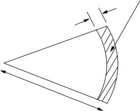
where σ◦ (θ) is the backscatter coefficient, as explained in Section 2.2.4, and Ac represents the clutter area. Figure 2.2 shows the scattering area, Ac, within the 3 dB beamwidth of the radar.
δR |
Clutter Area, Ac |
|
φ
R
Figure 2.2: Clutter Area in Azimuth Beamwidth and Pulse Duration Projected on the Ground.
2.2.4 Backscattering Coefficient σ◦
The backscattering coefficient, σ◦, used in Equation 2.9, is the radar cross section of a small increment of ground area, ∆A, and defined from [16] by,
σ0 |
= ΣN |
σn |
[m−2] |
(2.10) |
|
||||
m |
n=1 ∆A |
|
|
|
It defines an average radar cross section per unit area or the RCS of a distributed target of horizontal area A, normalized with respect to A. A reflector which concentrates its reflected energy over a limited angular direction may have an RCS for a particular direction which exceeds its projected area and hence backscattering coefficient and RCS are quoted with aspect angle.
2.2.5 The Radar Equation
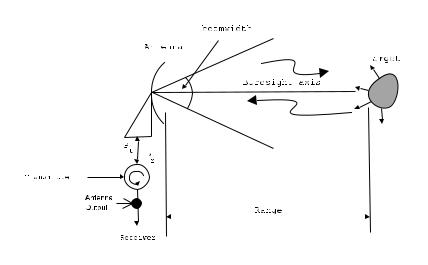
The radar equation relates the important parameters affecting the received signal of a radar. The derivation is explained in many texts, namely [6, pg11], [10, pg5], [12, pg7] and [14, pg198]. Figure 2.3 shows the backscattered power from a target with radar cross section, σt, at a range, R. The radar equation relating the range from the target to the
11
2.3. SAR BASICS |
|
|
|
|
CHAPTER 2. THEORY OF AIRBORNE SAR |
|||
|
|
|
|
|
|
|
|
|
|
|
|
|
|
|
|
|
|
|
|
|
|
|
|
|
|
|
|
|
|
|
|
|
|
|
|
|
|
|
|
|
|
|
|
|
|
|
|
|
|
|
|
|
|
Figure 2.3: Radar Backscatter From a Target.
radar is given by,
Prx = |
PtxG2λ2σt |
[W] |
(2.11) |
|
|||
|
(4π)3 R4Ls |
|
|
where Ls is the system losses. The radar equation is used to simulate the return power at the antenna output such that the maximum input power to the receiver is known.
2.3 SAR Basics
The platform on which the SAR is mounted is usually an aircraft or satellite. Figure 2.4 shows the stripmap SAR geometry and radar position relative to the ground. A burst of pulses is transmitted by a side-looking antenna pointed towards the ground and the backscattered power is collected with the signal corresponding to each pulse. The SAR system saves the phase histories of the responses at each position as the real beam moves past and then, in post processing it weighs, phase shifts and sums them up to focus on one point target (resolution element) at a time and suppresses all others.
2.3.1 Receiver Bandwidth
An important aspect in designing a radar is the radar bandwidth, Br. In conjuction with SAR, bandwidth will essentially mean the range of frequencies over which the target reflectivity data are collected. The receiver bandwidth is determined by the bandwidth of the transmitted pulse . The half power bandwidth of the radar receiver is the range of frequencies up to the point where the frequency response drops to half of its maximum and is known as the 3-dB bandwidth. The radar 3-dB bandwidth is related to the pulse
12