12-10-2013_09-24-50 / [Simon_Kendal,_Malcolm_Creen]_Introduction_to_Know(BookFi.org)

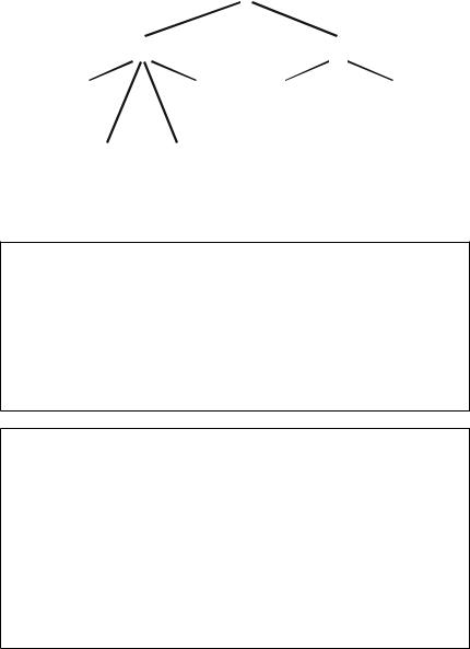
FIGURE 2.6. Learning by multi-layer perceptron.

The Back Propagation Algorithm

There is a difficulty in training a multi-layer perceptron network, i.e., how are the weights adjusted in the middle of the network. Thankfully back propagation, a well-known training algorithm solves this problem. It works in the following way:

1.An error value is calculated for each node in the outer layer.

2.The weights feeding into each node, in this layer, are adjusted according to the error value for that node (in a similar way to the previous example).

3.The error, for each of the nodes, is then attributed to each of the nodes in the previous layer (on the basis of the strength of the connection). Thus the error is passed back through the network.

4.Steps 2 and 3 are repeated, i.e., the nodes in the preceding layer are adjusted, until the errors are propagated backwards through the entire network, finally reaching the input layer (hence the term back propagation).

One minor complication remains—this training algorithm does not work when the output from a node can only be 0 or 1. A function is therefore defined that calculates the output of a neuron on the basis of its input where the output varies between 0 and 1.

A set of training data will be presented to the network one item at a time. Whenever the networks output is incorrect the weights are adjusted slightly as indicated. When all of the training data has been presented to the network once this is called an epoch (pronounced e-pok). An epoch will need to be presented to the network many times before training is complete.

FIGURE 2.7. Different artificial neural network architectures.

Activity 9

This activity will help you visualise a RBF network.

Visit the following URL: http://diwww.epfl.ch/mantra/tutorial/english/rbf/html/

The page contains a Java applet which demonstrates some function approximation capabilities of a RBF network

Follow the instructions on the web page.

Activity 10

This activity provides you with a second opportunity to work with a RBF network.

Visit the following URL: http://

www.mathworks.com/products/demos/nnettlbx/radial/

This is a series of illustrations showing how a neural network toolbox can be used to approximate a function. This demonstration uses the NEWRB function of the Matlab software (available from http://www.mathworks.com/) to create a radial basis network that approximates a function defined by a set of data points.

Self-Organising Maps

Although there has been considerably more progress in supervised learning research, Tuevo Kohonen has had some success with his development of a selforganising map (SOM). The SOM (also known as the Kohonen feature map) algorithm is one of the best-known ANN algorithms. Self-organising maps are a

data visualisation technique that reduces the dimensions of data through the use of self-organising NNs. In contrast to many other NNs using supervised learning, the SOM is based on unsupervised learning.

The way SOMs go about reducing dimensions is by producing a map of usually one or two dimensions that plot the similarities of the data by grouping similar data items together. So, SOMs accomplish two things, they reduce dimensions and display similarities.

Activity 10

A SOM applet—where data is represented by colour—is available at: http://davis.wpi.edu/ matt/courses/soms/applet.html

Try several iteration settings (e.g. 100, 500 and 1000) and compare the differences in accuracy of colour grouping.

The SOM is a unique kind of NN in the sense that it constructs a topology preserving mapping from the high-dimensional space onto map units in such a way that relative distances between data points are preserved. The map units, or neurons, usually form a two-dimensional regular lattice where the location of a map unit carries semantic information. The SOM can therefore serve as a clustering tool of highdimensional data. Because of its typical two-dimensional shape, it is also easy to visualise.

The first part of a SOM is the data. The idea of the SOMs is to project the n- dimensional data into something that is better understood visually. In the case of the applet you tried in the activity above, one would expect that pixels of a similar colour would be placed near each other. You might have found that the accuracy of arranging the pixels in this way increased the more iterations there were.

The second components to SOMs are the weight vectors. Each weight vector has two components: data and ‘natural location’. The good thing about colours—as in the SOM applet—is that the data can be shown by displaying the colour, so in this case the colour is the data, and the location is the position of the pixel on the screen. Weights are sometimes referred to as neurons since SOMs are a type of NNs.

The way that SOMs go about organising themselves is by competing for representation of the samples. Neurons are also allowed to change themselves by learning to become more like samples in hopes of winning the next competition. It is this selection and learning process that makes the weights organise themselves into a map representing similarities. This is accomplished by using the very

simple algorithm:

Initialise Map

For t from 0 to 1

Randomly select a sample

Get best matching unit

Scale neighbours

Increase t by a small amount

End for

The first step in constructing a SOM is to initialise the weight vectors. From there you select a sample vector randomly and search the map of weight vectors to find which weight best represents that sample. Since each weight vector has a location, it also has neighbouring weights that are close to it. The weight that is chosen is rewarded by being able to become more like that randomly selected sample vector. In addition to this reward, the neighbours of that weight are also rewarded by being able to become more like the chosen sample vector. From this step we increase t a small amount because the number of neighbours and how much each weight can learn decreases over time. This whole process is then repeated a large number of times, usually more than 1000 times.

In the case of colours, the program would first select a colour from the array of samples such as green, then search the weights for the location containing the greenest colour. From there, the colours surrounding that weight are then made more green. Then another colour is chosen, such as red, and the process continues (see Figure 2.8).

Activity 11

This activity will help you visualise the concept of SOMs.

Nenet (Neural Networks Tool) is a Windows application designed to illustrate the use of a SOM. Self-organising map algorithm is categorised as being in the realm of NN algorithms and it has been found to be a good solution for several information problems dealing with high-dimensional data.

1.Visit the Nenet Interactive Demonstration page at: http://koti.mbnet.fi/ phodju/nenet/Nenet/InteractiveDemo.html.

2.Click on the ‘Open the demonstration’ link.

3.Proceed through the demonstration, reading the onscreen explanations as you do so.

You may also wish to download and install the demonstration version of Nenet which has the following limitations on the data and map sizes:

Maximum map size: 6 × 6 neurons.

Maximum number of data vectors: 2000.

Maximum data dimension: 10.

FIGURE 2.8. Self-organising map after 1000 iterations.

SOMs Reducing Dimensions—What Does This Mean

in Practise?

Imagine a new celebrity becomes very famous and their face is shown on television, on large posters and in the press. Having seen their face on several occasions you begin to recognise their features. You won’t remember every detail and every pixel of a high resolution photograph but the essential features will be stored in your brain. On seeing a new high resolution photograph your brain will pick out the same essential features and compare them with the details stored in your memory. When a match occurs you will recognise the face in the photograph. By storing only the essential features your brain has reduced the complexity of the data it needs to store.

Why is This Unsupervised Learning?

For many of the things you learn there is a right and wrong answer. Thus if you were to make a mistake a teacher could provide a correct response. This is supervised learning. SOMs group similar items of data together. When picking out the features of a face various features can be chosen, eye colour, the shape of the nose etc. The

features you pick can affect the efficiency of the system but there is no wrong or right answer—hence this task is an example of unsupervised learning.

Other examples of SOMs available on the Internet are:

The World Poverty Map at: http://www.cis.hut.fi/research/som-research/ worldmap.html

WEBSOM—SOMs for Internet exploration at: http://websom.hut.fi/websom/

Using ANNs

In the previous activity, you observed a demonstration of a NN—in the form of a SOM. You should have noted a definite sequence of steps in the process.

Activity 12

This activity helps you recognise the significant stages in the process of applying a NN to data analysis problems.

Write down what you consider to be the main stages in the demonstration of the Nenet software when applied to the example problem illustrated in the demo.

Under what circumstances could one of the stages has been skipped?

Why is this possible?

How is ‘Training Length’ measured?

Feedback 12

You should have been able to identify the following stages:

Initialise a new map

Set initialisation parameters

Train the map to order the reference vectors of the map neurons (not if using linear initialisation)

Train the map (again)

Test the map

Set test parameters.

Had linear initialisation type been selected, the first training step could have been skipped.

The training process could be run twice. The first step is to order the reference vectors of the map neurons. The linear initialisation already does the ordering and that is why this step can be skipped.

Training length is the length of the training measured in steps, each corresponding to one data vector. If the specified number of steps exceeds the number of data vectors found in the file, the set of data is run through again.

Choosing a Network Architecture

Although certain types of ANN have been engineered to address certain kinds of problems, there exist no definite rules as to what the exact application domains of ANNs are. The general application areas are:

robust pattern recognition

filtering

data segmentation

data compression

adaptive control

optimisation

modelling complex functions

associative pattern recognition.

Activity 13

Search the Internet for references to the Hopfield Associative Memory Model.

You will find a page containing some Java applets illustrating the Hopfield model at:http://diwww.epfl.ch/mantra/tutorial/english/hopfield/html/

and the Boltzmann machine at:http://www.cs.cf.ac.uk/Dave/JAVA/boltzman/ Necker.html

Run the applets with different parameters.

Figure 2.9 shows how some of the different NN architectures have been used.

FIGURE 2.9. The use of well-known neural networks.

Benefits and Limitations of NNs

The benefits of NNs include the following:

Ability to tackle new kinds of problems. Neural networks are particularly useful at finding solutions to problems that defeat convention systems. Many decision support systems now incorporate some element of NNs.

Robustness. The networks are more used to dealing with less structured problems.

The limitations of NNs include:

Artificial neural networks perform less well at tasks humans tend to find difficult. For example, they are less good at processing large volumes of data or performing arithmetical operations. However, other programs are good at these tasks and so they compliment the benefits of ANNs.

Lack of explanation facilities. Unlike many expert systems, NNs do not normally include explanation facilities making it difficult to determine how decisions were reached.

Test data. ANNs require large amounts of data. Some of the data is used for training and some to ensure the accuracy of the network prior to use.

Condition Monitoring

Condition monitoring is the name given to a task for which NNs have often been used, but what is it?

Every car driver listens to the noises made by their car. The noises will change depending upon many things:

the surface of the road

whether the road is wet or dry

the speed the car is going

the strain the engine is under.

While the car makes a range of normal noises other noises could indicate a problem that needs to be addressed. For example a tapping noise can indicate a lack of oil. If this is not rectified serious and expensive damage could be caused to the engine. Over time car drivers become familiar with the noises their car makes and will mostly ignore them until an unusual sound occurs. When this does occur a driver may not always be able to identify the cause but if concerned will get their car checked by an engineer. This allows maintenance to be carried out before serious damage occurs.

In the example above condition monitoring is something that the car driver is subconsciously doing all of the time—i.e., by listening to the noises the car makes they are monitoring the condition of the car and will initiate maintenance when required.

Just as a car requires maintenance so do many machines. Businesses, factories and power plants depend upon the correct functioning of a range of machines including, large extractor fans, power generators and food processors. Catastrophic failure in a large machine can in some cases cause an entire business to close down while repairs are made. Clearly, this is not an option and thus to prevent this regular maintenance is carried out. But to maintain a machine means shutting it down and even for short periods this becomes an expensive business. There is therefore a

FIGURE 2.10. A vibration spectra.

desire is to maintain the machine when it is required but not on a regular basis. However, how do we know when maintenance is required? One option is to monitor the condition of the machine. By fitting vibration detectors to the machine we can collect vibration spectra (see Figure 2.10).

Collecting vibration patterns is the equivalent to listening to a car however most machines, just like cars, make a range or normal noises. How do we therefore identify when a machine is developing a fault that requires maintenance?

Neural networks have in recent years been applied quite successfully to a range condition monitoring tasks. Neural networks are adept at taking in sensory data, e.g. vibration spectra and identifying patterns. In this case the network can learn which spectra represent normal operation and which indicates a fault requiring attention.

While NNs may appear to be the obvious solution to this task there are other options that could be considered. Interface Condition Monitoring Ltd. (UK) is a company that specialises in undertaking this sort of analysis. With years of experience in this field they decided to try and capture some of their knowledge in order to benefit trainee engineers. Working with the University of Sunderland (UK) they decided to capture this knowledge in an expert system. While the development of an expert system was possible there were some programming hurdles that needed to be overcome. Expert systems, unlike NNs, are not adept at processing sensory information. Thus before the expert system could make decisions the spectra needed