Cramer C.J. Essentials of Computational Chemistry Theories and Models

Reaction coordinate

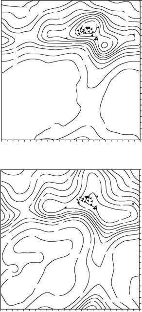
Figure 13.2 Schematic comparison of gas-phase and aqueous dipole moments (- - - - - -) to the free energy of solvation ( ) along the reaction path for the Claisen rearrangement as computed at the QM/MM level. FEP technology allows access to the solvation free energy, while the QM treatment of the substrate permits evaluation of the dipole moment operator. Note the large increase in polarizability (as judged by the difference between gas-phase and aqueous dipole moments) in the region of the TS structure that contributes to a sharp increase in the magnitude of the favorable solvation free energy. Note also, however, that comparison of the relevant curves indicates that the total solvation free energy depends on more than just the dipole moment

the QM solute charge distribution could be directly analyzed. As illustrated in Figure 13.2, Gao found that the polarizability of the Claisen substrate was substantially larger in the region of the transition state (as judged by the induced dipole moment attributable to solvation), and that this contributed significantly to increasing the favorable relative solvation free energy of the TS structure compared to the reactants, thereby adding to rate acceleration. The same inference was made from analysis of pure QM continuum model results, but without an ability to correlate polarizability with hydrogen bonding propensity.

Of course, the rich information available from a QM/MM simulation does not come without cost. The QM/MM Claisen simulation required several million AM1 calculations to be carried out; while AM1 is a very efficient level of QM theory for a molecule as small as allyl vinyl ether, that still represents an enormous investment of computational resources. As a result, the application of QM/MM methodologies based on the formalism of Eqs. (13.4) and (13.5) has tended not to be especially systematic, i.e., choices of QM and MM models and necessary coupling parameters have tended to be made on an ad hoc basis, without regarding parameter transferability as being an issue of paramount concern.

With increasing use of such models, methods are likely to become more concisely defined in the near future. At present, the models for which protocols and parameters have been most clearly defined and where a fair number of applications have appeared applying those models in a consistent fashion include the already noted AM1/TIP3P model (more generally AM1/OPLS when solvents other than water are employed in the MM region) and a similarly fashioned HF/3-21G/OPLS model (Freindorf and Gao 1996). Implementations carrying the QM level as far as coupled-cluster theory have been reported (Kongsted et al. 2003).

A variation on the QM/MM theme that offers an increase in computational speed by sacrificing a certain level of microscopic detail has seen a moderate level of application when the MM system is simply a homogeneous solvent. In such cases, explicit atomistic representation of the solvent molecules is replaced with a set of integral equations governing their mutual interaction, for example, the reference interaction site model (RISM; Pratt and Chandler 1977). The equations are quite complex (and their solution can be a challenging numerical task) but in essence integral equation theories take as input the force-field parameters and interaction potentials associated with a molecular mechanics solvent molecule (e.g., TIP3P water or OPLS chloroform), and they output radial distribution functions describing the solvent’s average structure (see Section 3.5). Alternatively, Freedman and Truong (2003) have described using RISM with solvent r.d.f.s computed from explicit simulations. In any case, integral equation models are in some sense intermediate between continuum models, which include no solvent structural information, and explicit models, where individual snapshots of a solvated system comprise the data from which averages are computed.

Several models combining QM solute representations with a RISM solvent treatment have been described recently. The QM solute is described as a sum of site potentials just as the MM solvent is, except that the electrostatic portion of the potentials derives from the QM wave function. Using the radial distribution functions for solvent charge sites about solute atoms permits the solvent electrostatic influence on the QM wave function to be determined. The RISM equations are then solved for the full set of site potentials until self-consistency is reached (Ten-no, Hirata, and Kato 1993). Given the final site –site distributions and the interaction potential between all sites, it is possible to compute the free energy of solvation (Lee and Maggiora 1993). In a QM/RISM hybrid model, experimental data for this quantity may be used to optimize LJ parameters for QM atoms, and this approach has been used to define the hybrid extended RISM and quantum mechanical solvation model XSOL (Shao, Yu, and Gao 1998) for use in modeling organic equilibria in aqueous solution.

Rather than treating the entire solvent via the RISM formalism, an alternative approach that has seen some study is to represent some solvent molecules explicitly, typically as MM species, and then embed the entire QM/MM cluster in a continuum dielectric medium according to the formalisms described in Chapter 11. Both Bandyopadhyay et al. (2002) and Cui (2002) adopted such an approach to study the neutral/zwitterionic equilibrium of glycine in water, the former group representing the explicit water molecules with the EFP model and Cui doing so with a modified TIP3P model. Both studies concluded that inclusion of some explicit solvent molecules gave critically improved accuracy over modeling the problem with exclusively continuum solvation. Note that inclusion of specific MM solvent molecules

about a QM anion has the additional benefit of substantially reducing any likely instabilities associated with charge penetration (see Section 11.4.1.3).

13.2.3Fully Polarized Interactions

Allowing the QM system to be polarized by the MM charges without at the same time accounting for polarization of the molecules comprising the MM system may be regarded as being possibly unbalanced. One approach for including polarizability in the MM system has already been described in Chapter 12, and its extension to a QM/MM system is algorithmically trivial. Thus, each MM molecule or atom is assigned a polarizability tensor α, and the induced dipole at each polarizable center is determined from Eq. (12.30); in the QM/MM system, the electric field E has the same components from the MM partial charges and induced dipoles as in a fully classical system, and an additional component deriving from the nuclei and electronic wave function of the QM system that is straightforward to calculate. The interaction of the induced dipoles with the MM partial charges (Eq. (12.31)) and with one another (Eq. (2.23)) are added in the HMM term of Eq. (13.1). In addition, the induced dipoles interact with the nuclei of the QM system according to Eq. (12.31), and with the electronic wave function as the expectation value of the operator equivalent of Eq. (12.31) (thereby adding additional one-electron integrals to the Fock operator, one for each induced dipole).

The evaluation of all of these terms must proceed iteratively until self-consistency is reached, since the induced dipoles and the relaxing QM wave function modify the electric field on which the induced dipoles are dependent. Thus, the increase in computational resources required to include MM polarizability can be quite significant – one order of magnitude is not uncommon. Comparisons between QM/MM systems modeled with and without MM polarizability have been largely equivocal on the utility of its inclusion (adding alternative three-body correction terms has also been examined for the hydrated manganous ion (Loeffler, Yague, and Rode 2002) and was similarly found to lead to no significant improvement in describing hydration structure). Given its very high cost of implementation, there seems to be little point in carrying the model to this degree of physicality. However, the lack of improvement in many cases may be attributable to the polarizability being added post facto to an already existing force field. By virtue of fitting to experiment, formally nonpolarizable force fields must include polarization in some average way into their parameters, making it less likely that additional explicit accounting for polarization will show dramatic effects. It is likely that only ongoing efforts aimed at developing fully polarizable force fields from scratch will prove definitive in determining the level of additional physical insight that may be gained from having polarization present in explicit form (see, for instance, Banks et al. 1999).

Although complete, fully polarizable QM/MM schemes are computationally demanding, a simplified version of this formalism was arguably the first QM/MM approach to be described (Warshel and Levitt 1976), and the method still sees some use today. The simplification involves replacing explicit, polarizable MM molecules with a three-dimensional grid of fixed, polarizable dipoles – each a so-called Langevin dipole (LD) as it is required to obey

the Langevin polarization law. Each dipole enters the Fock operator just as described above (Luzhkov and Warshel 1992).

Much like the RISM method, the LD approach is intermediate between a continuum model and an explicit model. In the limit of an infinite dipole density, the uniform continuum model is recovered, but with a density equivalent to, say, the density of water molecules in liquid water, some character of the explicit solvent is present as well, since the magnitude of the dipoles and their polarizability are chosen to mimic the particular solvent (Papazyan and Warshel 1997). Since the QM/MM interaction in this case is purely electrostatic, other nonbonded interaction terms must be included in order to compute, say, solvation free energies. When the same surface-tension approach as that used in many continuum models is adopted (Section 11.3.2), the resulting solvation free energies are as accurate as those from ‘pure’ continuum models (Florian´ and Warshel 1997). Unlike atomistic models, however, the use of a fixed grid does not permit any real information about solvent structure to be obtained, and indeed the fixed grid introduces issues of how best to place the solute into the grid, where to draw the solute boundary, etc. These latter limitations have curtailed the application of the LD model.

13.3 Boundaries Through Bonds

All of the QM/MM models discussed this far, much like continuum models, envision partitioning a chemical system into (at least) two distinct regions, where the boundary between these regions is everywhere characterized by a very low level of electron density. That is, no atoms on one side of the boundary are bonded to atoms on the other side. As a result, the HQM/MM term in the Hamiltonian of Eq. (13.1) is restricted to non-bonded interactions.

The situation is vastly more complicated when the boundary between the QM and MM regions passes across one or more chemical bonds. Somehow, the dangling valences from the two separate regions must be joined in a chemically (and computationally) sensible fashion. Developmental work is ongoing in this area; this section will focus on the current most widely used procedures.

13.3.1Linear Combinations of Model Compounds

Many efforts in molecular design make use of sterically demanding groups, e.g., t-butyl groups, to enforce particular molecular geometries. Viewing the total molecule as some kind of sum of its functional groups, the intent is for the interaction between the large groups and the remainder of the molecule to be entirely steric in nature. In such a situation, the inclusion of the bulky group(s) in a fully QM calculation may be regarded as pointlessly expensive, since the size of the fragment(s) guarantees a large increase in the total number of QM basis functions, but the non-polarity of the fragments also indicates little likelihood of perturbing the electronic structure of the remainder of the molecule via electrostatic interactions (steric interactions are, of course, fundamentally electronic exchange-repulsion interactions, but for the moment we will ignore this level of detail and consider steric effects to be distinct from more classical electrostatic interactions). Thus, there is a clear motivation for passing a

QM/MM boundary through space in such a way that the sterically bulky groups fall on the MM side and the ‘interesting’ part of the molecule falls on the QM side. Finally, to avoid the question of how to deal with a cut bond, one may assume that the electronic structure of the QM region will be of similar quality with either the non-polar, bulky group as a cap, or with simply hydrogen atoms as caps. With such a philosophy, the energy of the system as a whole may be expressed as a linear combination of model compounds of different size and at different levels of theory. In simplest form

where the large system is the complete molecule, which is only treated at the MM level of theory, and the small system is the ‘core’ portion whose electronic structure is of primary interest, and it is computed at both the MM and QM levels. The two different term orderings on the r.h.s. of Eq. (13.6) are meant to emphasize the two primary motivations for pursuing this decomposition of the Hamiltonian.

The first motivation has already been emphasized above. There is some reason to believe that all of the important quantum effects are captured in the small system, and the steric energy associated with the bulky groups will be well captured as an ‘embedding’ energy, i.e., the difference between the MM energy of the small system and the large system. For example, Cramer and Pak (2001) modeled the reaction coordinate for intramolecular C –H bond cleavage from a benzyl position in [(LCu)2(µ-O)2]2+, L = 1,4,7-tribenzyl-1,4,7- triazacyclononane, by replacing the five non-reactive benzyl groups with H atoms in the small model system (Figure 13.3). As this QM system was treated at the density functional level

Figure 13.3 A bis(µ-oxo)dicopper complex represented using Eq. (13.6) where each boxed R group is H for the small QM system and benzyl for the large MM system. The structure on the right is a TS structure for H-atom transfer from C to O found by optimization at the hybrid level of theory. All other H atoms have been removed for clarity

of theory with a double-ζ basis set, reducing the system by 35 heavy atoms and 30 hydrogen atoms substantially reduced the total number of basis functions. The necessary MM energies were then computed with the UFF force field. Application of the model in this fashion has been especially attractive within the organometallic community, where large ligands can often be regarded as having a core portion that is electronically important, and remaining regions that are not. Thus, for example, Matsubara et al. (1996) have used combined DFT/MM models to study dihydrogen activation by platinum with different phosphine ligands, and Deng et al. (1997) have used other DFT/MM models to study the role of bulky substituents in Brookhart-type Ni(II) diimine-catalyzed olefin polymerization.

The alternative motivation for the second equality of Eq. (13.6) arises in cases where a force field may be regarded as being reasonably accurate except perhaps for some specific quantum mechanical effect(s) not well accounted for in the functional form of the force field. For example, French et al. (2000) constructed a (φ,ψ) potential energy surface for the torsions about the anomeric linkages in sucrose by adjusting an MM3 surface for the full molecule based on the difference between HF/6-31G(d) and MM3 surfaces for a tetrahydropyrantetrahydrofuran ether model (i.e., sucrose without any hydroxyl groups, Figure 13.4). The MM3 force field exhibits a weakness in accounting for the so-called ‘anomeric effect’ in sugars (see Section 2.2.3). By correcting for this weakness using the QM results, French et al. were able to demonstrate that a sizable number of crystal structures containing sucrose moieties that had previously been assumed to be adopting abnormally high-energy conformations were instead in low-energy regions of the surface.

Note that the embedding philosophy of Eq. (13.6) may be applied more generally than simply in the context of QM/MM calculations. For example, one can imagine situations where the importance of a high-level accounting for electron correlation effects may be restricted to a small region of a large system, but the full system still requires an overall QM treatment. In such an instance, two different QM levels might be used in Eq. (13.6) instead of one QM and one MM level; obviously, the more efficient QM level is the one applied to the large system. For example, Sherer and Cramer (2001) studied the context dependence of the pKa of the cytosine:2-aminopurine base pair in different double-helical RNA trimers by taking the base pair itself to be the small system and the trimer to be the large system, and choosing as the high and low levels of theory MP2/6-31G(d) and PM3, respectively, each augmented with an aqueous continuum solvation model (Figure 13.5).

Note that Eq. (13.6) is written in terms of energies and not Hamiltonian operators. That is because there is a certain ambiguity about how to define a wave function that would be simultaneously appropriate for all of the Hamiltonian operators that would otherwise appear on the r.h.s. This is not purely a notational issue, since it leaves open the question of the geometries used for the different energy terms. For instance, one approach would be to consider each energy on the r.h.s. to refer to complete geometry optimization at the appropriate level. This is clearly the simplest method, since every energy determination may be carried out completely independently of the others. However, if there are large differences between the corresponding regions of any pair of geometries, it calls into question the validity of the overall energy expression.

frozen region

Figure 13.5 An application of a hybrid MO/MO philosophy to the indicated RNA trimer proceeds using correlated levels of electronic structure theory for various tautomers and protonation states of the central base pair, this pair then representing the small system in the MO/MO analog of Eq. (13.6), and semiempirical theory for both the small system and the frozen-geometry larger system

An alternative is to force those atoms common to the large and small models (i.e., all of the atoms in the small model except the capping hydrogens) to occupy the same coordinate locations in all three energy evaluations. Within this set of restraints, one may then write down fairly simple expressions for the gradients as sums of QM and MM gradients from the small and large systems, noting that there are some details associated with the capping atoms in the small system and the alignment of bonds to capping atoms with bonds in the full system (see, for example, Vreven et al. 2003 and Swart 2003). Maseras and Morokuma (1995) were the first to provide such gradient expressions, referring to the optimization approach as the integrated molecular orbital molecular mechanics method (IMOMM).

Subsequently, Humbel, Sieber, and Morokuma (1996) generalized the IMOMM optimization scheme to the case where two different levels of QM theory were used instead of a QM/MM approach, and Svensson, Humbel, and Morokuma (1996) examined the relative efficacy of different combinations of levels for prototype problems. Corchado and Truhlar (1998) later proposed a refinement of that methodology to improve computed vibrational frequencies and Rickard et al. (2003) showed that a combination of MP2 and HF theories permits the calculation of high-quality NMR chemical shifts within the high-level system.

Of course, Eq. (13.6) admits to further generalization. Rather than dividing a system into large and small models, there may be instances where a division into large, medium, and small models may be advantageous, with increasingly smaller regions treated with increasingly higher levels of theory. Svensson et al. (1996) generalized their geometry optimization scheme to this more general case, demonstrating the method for MO/MO/MM combinations, and refer to it as ONIOM, where the acronym, representing ‘our own n-layered integrated molecular orbital molecular mechanics’ scheme, is meant to emphasize the typical inward- to-outward, near-spherical layering of models that is typically chosen and is reminiscent of the almost eponymous lachrymatory bulb. To provide yet another layer of modeling when condensed-phase effects are of interest, the combination of ONIOM with the PCM continuum solvation model has been described (Vreven et al. 2001) as has a model for permitting explicit solvent molecules to morph from MM to QM while passing through a buffer region surrounding the QM subsystem (Kerdcharoen and Morokuma 2002).

13.3.2Link Atoms

Situations arise where the influence of the MM region on the QM region to which it is bonded cannot be regarded simply as steric. In a large protein, for instance, polar and possibly charged residues in an MM region inevitably will polarize a QM region in the same protein. The only way to eliminate such QM/MM coupling is to include the entire protein in the QM region, and such an approach is extremely impractical for anything other than a possible single-point calculation at a fairly low level of electronic structure theory.

Of course, the strong coupling invoked here between the two regions is in no manner different than that dealt with in Section 13.2.2. What is different is that now there are interaction energy terms between the QM and MM regions that are not non-bonded terms, these new terms being associated with the bonds cut by the QM/MM boundary. In practice, coupled QM/MM calculations involving link atoms tend to adopt the following protocols for computation of the various terms.

1.HQM is computed for the QM region capped with hydrogen atoms at every bond cut by the QM/MM boundary. The Fock operator may be like that defined in Eq. (13.5). However, since the capping hydrogen atom is not really a part of the system, the third term on the r.h.s. is not evaluated when µ or ν is a basis function on a capping hydrogen; similarly, no nuclear repulsion between the capping hydrogen nucleus and the MM atoms is computed.

2.The energies of bonds cut by the QM/MM boundary are evaluated using the standard MM bond-stretching term (i.e., as though the QM atom were an MM atom). In addition, a very large force constant is applied to the fictitious bond angle MM–atom–QM–atom–capping–H so that it remains essentially zero (note that this connectivity choice avoids the difficulty of working with bond angles near π radians).

3.Angle bending energies involving two MM atoms and one QM atom are computed using the standard force-field formulation. Angle bending terms involving one MM atom and