Cramer C.J. Essentials of Computational Chemistry Theories and Models

384 10 THERMODYNAMIC PROPERTIES

Cloud, C. F., III, and Schwartz, M. 2003. J. Comput. Chem., 24, 640. Cossi, M. and Crescenzi, O. 2003. J. Chem. Phys., 118, 8863.

Fishtik, I., Datta, R., and Liebman, J. F. 2003. J. Phys. Chem. A, 107, 695. Hout, R. F., Jr., Levi, B. A., and Hehre, W. J. 1982. J. Comput. Chem., 3, 234. Irikura, K. K. 2002. J. Phys. Chem. A, 106, 9910.

Jensen, F. 2003. Mol. Phys., 101, 2315.

Moore, C. 1952. Natl. Bur. Stand. (US), Circ. 467.

Ochterski, J. W., Petersson, G. A., and Wiberg, K. B. 1995. J. Am. Chem. Soc., 117, 11299. Pitzer, K. S. and Gwinn, W. D. 1942. J. Chem. Phys., 10, 428.

Saraf, S. R., Rogers, W. J., Mannan, M. S., Hall, M. B., and Thomson, L. M. 2003. J. Phys. Chem. A, 103, 7900.

Winget, P. and Clark, T. 2004. J. Comput. Chem., 25, 725.

Zhao, Y., Lynch, B. J., and Truhlar, D. G. 2004. J. Phys. Chem. A, 108, 4786.

11

Implicit Models for Condensed Phases

11.1 Condensed-phase Effects on Structure and Reactivity

The gas phase is delightful in its simplicity. At low to moderate pressures, molecules may be treated as isolated, non-interacting species, and this facilitates theoretical modeling enormously, insofar as the system of interest is entirely defined by the molecule itself. Were theory to restrict itself to the gas phase, however, it would be inapplicable to vast tracts of chemistry, to include essentially all of biochemistry.

Of course, one can carry out accurate gas-phase calculations and then make broad generalizations about how one might expect a surrounding condensed phase to affect the results. Indeed, this modus operandi was much employed well into the 1980s and still sees modest use today. Provided one can be reasonably confident that condensed-phase effects are small for the particular properties being studied (either in an absolute sense or through cancellation by judicious comparisons), such an approach can still be useful, particularly in a qualitative sense. However, significant developmental efforts over the last two decades combined with growth in the computational power required to implement them have resulted in the widespread availability of condensed-phase models designed to more accurately describe the physical nature of condensed-phase systems. This chapter considers one such class of these models, namely, implicit solvation models, which are also often called continuum solvation models.

At first thought, of course, it might seem that the modeling of a condensed-phase system should be trivial. Take for example a liquid solution (which we will take as our ‘default’ condensed phase in this and the next chapter, although others will be discussed). If our solution is dilute, then the ‘obvious’ way to construct a model is to surround our solute with a number of solvent molecules. But a critical question is, how many? If we want to consider glucose in water, for instance, it seems clear that we would want at least the entire surface of the glucose molecule to be covered. This might take, say, 14 water molecules, which we could place approximately at the corners and faces of an imaginary cube about our solute. However, it would be something of a stretch of faith to imagine this as true aqueous solvation – none of the water molecules is interacting with a second solvation

Essentials of Computational Chemistry, 2nd Edition Christopher J. Cramer

2004 John Wiley & Sons, Ltd ISBNs: 0-470-09181-9 (cased); 0-470-09182-7 (pbk)

shell, making many otherwise plausible hydrogen bonding arrangements inaccessible. So, we might add another solvation shell. Since the surface area of a sphere increases as the square of the radius, it is clear that we will need many more than 14 waters this time. Will two solvation shells be enough? Almost certainly not – to eliminate spurious ‘edge’ effects associated with the water molecules on the outside, we really should add hundreds or thousands of waters. But if we do so, our system size becomes enormous – a quantum mechanical calculation on a single geometry will be staggeringly expensive. Worse still, that single geometry is of very limited value. As noted in Chapter 3 and discussed further in Chapter 12, with so many molecules and so many possible minima we need to compute statistical mechanical averages in order to determine equilibrium properties. Thus, we need to carry out possibly millions of these staggeringly expensive quantum calculations, and such a situation is simply not practical within the confines of present resources.

The assumption underlying continuum solvation models, which are the subject of this chapter, is that one may remove the huge number of individual solvent molecules from the model, as long as one modifies the space those molecules used to occupy so that, modeled as a continuous medium, it has properties consistent with those of the solvent itself. To determine how to define such a medium, one must consider the solvation process itself.

11.1.1Free Energy of Transfer and Its Physical Components

The most important fundamental quantity describing the interaction of a solute with a surrounding solvent is the free energy of solvation GoS. This quantity is sometimes also called the free energy of transfer, and refers to the change in free energy for a molecule A leaving the gas phase and entering a condensed phase. This free energy may be determined from the equilibrium constant describing the partitioning of A between the gas and condensed phases according to

where the limit is applied to ensure ‘ideal solution’ behavior. As with all free-energy quantities, attention must be paid to the standard-state concentrations. Most theoretical work makes use of standard-state concentrations of 1 M in both the gas phase and the condensed phase. In that case, there is no intrinsic change in the entropy of translation of the solute associated with a change in standard-state volume. Common experimental conventions, however, include expressing the gas-phase concentration as a partial pressure, with 1 atm defining the standard state, and/or expressing the solution concentration as mole fraction, with unit mole fraction defining the standard state (conversion between different concentration standard states for free energies of solvation can be accomplished using Eq. (10.53) in the same fashion already described for reaction equilibrium constants).

Experimental free energies of solvation span a wide range of values, from positive tens to negative hundreds of kilocalories per mole (for those values where the solution/gas equilibrium constants fall outside the range of about 10−6 to 106, experimental techniques other

than simply measuring the concentrations in the two distinct phases are typically required). Different physical effects contribute to the overall solvation process; of these, the most important components are electrostatic interactions, cavitation, changes in dispersion, and changes in bulk solvent structure.

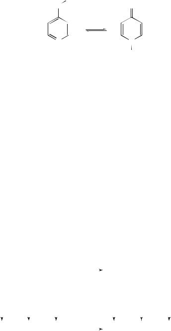
Equilibrium electrostatic interactions between a solute and a solvent are always nonpositive – they are zero if the solute is characterized by no electrical moments (e.g., a noble gas atom) and negative otherwise, i.e., attractive. It is easiest to visualize the electrostatic interactions as developing in a stepwise fashion. Consider a solute A characterized by electrical moments; for simplicity, consider only the dipole moment. When A passes from the gas phase into a solvent, the solvent molecules, if they have permanent moments of their own, reorient so that, averaged over thermal fluctuations, their own dipole moments oppose that of the solute. In an isotropic liquid with solvent molecules undergoing random thermal motion, the average electric field at any point will be zero; however, the net orientation induced by the solute changes this, and the field induced by introduction of the solute is sometimes called the ‘reaction field’.

Of course, the presence of an electric field means that a term accounting for the interactions of charged particles with this field should be included in the solute Hamiltonian. When it is included, the effect is to increase the solute polarity in a fashion proportional to the solute polarizability and the strength of the external field. Thus, the dipole moment of A increases. The solvent, seeing this increase, itself polarizes and moreover increases its own orientation to oppose A’s dipole, and so on.

However, neither the orientation/polarization of the solvent nor the electronic polarization of A is without cost. In the first instance, since solvent molecules are oriented to oppose the dipole moment of A, they each interact in an unfavorable sense with the reaction field they create. Moreover, to the extent they have lost some configurational freedom, there is an associated free-energy cost. As for the cost of electronic polarization, this may be viewed as the gas-phase cost (as computed with the gas-phase Hamiltonian) associated with distortion of the wave function away from the gas-phase minimum. As a result of these opposing energetics, the polarization of the solute/solvent system stops at that point where any energy gain from additional polarization is exactly balanced by the energy cost to achieve that polarization. Under some fairly mild assumptions from so-called linear response theory, one can show that this occurs when the energy cost up to a certain point becomes equal to one half of the total interaction energy between the solute and the solvent.

It cannot be overemphasized that solvation changes the solute electronic structure. As noted above, dipole moments in solution are larger than the corresponding dipole moments in the gas phase. Indeed, any property that depends on the electronic structure will tend to have a different expectation value in solution than in the gas phase. How large will the difference be? That depends on the strength of the solute –solvent interactions. Table 11.1 lists dipole moments computed in the gas phase, chloroform, and water for six nucleic acid bases at the HF/6-31G(d) level using the SM5.42R continuum solvation model that is described in more detail below. Note that the increases in dipole moments on going from the gas phase to water range from about 25 to 33 percent for these molecules; a smaller but still substantial increase is predicted in chloroform solution.

Another physical effect associated with solvation is cavitation. It is again helpful to visualize the solvation process as a stepwise procedure. Here, we imagine the first step as being creation of a cavity of vacuum within the solvent into which the solute will be inserted as a second step. The energy cost of the cavity creation is the cavitation energy. Note that energy is always required to create the cavity – if it were favorable to create ‘bubbles’ of vacuum in the liquid, the solvent would not remain in the liquid phase.

As for what holds liquids together in the first place, the majority of the interaction energy in uncharged fluids derives from dispersion forces between solvent molecules that are in contact with one another. This is true even for liquids composed of very polar molecules: dispersion accounts for 70–90 percent of the total cohesion energy in liquid HCl or 2-butanone. Recalling the discussion in Section 2.2.4, dispersion refers to the always favorable interaction between the simultaneous induced dipoles in adjacent molecules that are a consequence of the correlated motion of electrons. When a solute is inserted into a pre-existing cavity into which it exactly fits, it will experience favorable dispersion interactions with the surrounding solvent. Note that while formally dispersion is an electrostatic interaction, it is usually discussed separately from the solute –solvent polarization described above in deference to its short-range character and its non-classical origin. Note also that it is dispersion alone that can account for a favorable transfer free energy of a solute into a solvent when neither of the two is characterized by any permanent electrical moments.

Finally, under certain conditions, the introduction of a solute molecule may significantly alter the equilibrium structure/dynamics of a solvent in the near vicinity of the solute, and this phenomenon will have associated with it a free-energy change. The most widely documented example is the hydrophobic effect, where loss of orientational freedom for water molecules in the first solvation shell about hydrocarbon fragments of solutes carries with it a free-energy cost that is responsible for the increasingly positive aqueous free energies of solvation of alkanes as they increase in chain length.

Having enumerated the various processes involved in the transfer of a solute molecule from the gas phase to solution, it must be emphasized that it is not possible to separately measure their contributions to the fundamental observable, GoS. One can, of course, attempt to design systems where one expects only a single contribution to dominate, in the hopes of learning more about the nature of that contribution from experimental measurements, but inferences drawn therefrom become less certain as they are applied to systems less like those originally

measured. This point is made insofar as we will discuss below, for example, theoretical predictions for the electrostatic component of the free energy of solvation. However, insofar as this quantity is not an experimental observable, absolute judgments of quality comparing one level of theory to another are necessarily model-dependent.

11.1.2Solvation as It Affects Potential Energy Surfaces

In order to visualize the effects of solvation on structure and reactivity, it is helpful to consider the potential energy surface created by adding the free energy of solvation point by point to the gas-phase PES, as illustrated in Figure 11.1. (To be rigorous, one really should use a gas-phase free-energy surface so as not to be haphazardly mixing potential and free energies, but for qualitative purposes, we may ignore this technical point.) Processes in solution may be regarded as occurring on the lower surface, and all of the phase-space dimensions associated with solvent molecules have been averaged over in computing its energies.

Figure 11.1 illustrates several critical concepts associated with solvation. First, note that the reaction process depicted on the gas-phase surface joins two minima of roughly equal energy, while that on the lower surface is quite exergonic in the left-to-right direction. This derives from the minimum-energy structure at the larger x coordinate having a more negative free energy of solvation. Differential solvation of two (or more) minima implies a different equilibrium constant in solution than in the gas phase. Many examples of this

gas-phase surface

∆G oS(x,y)

E

solvated surface

(x,y)

Figure 11.1 A two-dimensional gas-phase PES and the corresponding PES derived from adding the free energy of solvation to every point. This process is illustrated for point (x,y). Thick lines on the two surfaces indicate some chemical reaction proceeding from one minimum-energy structure to another. Note that there is no requirement for the x and y coordinates of equivalent stationary points on the two surfaces to be the same

the process in solution, one need only take appropriate sums and differences of the upper horizontal leg and the vertical legs, viz.

As the upper leg is a gas-phase quantity, it can be computed taking advantage of all of the technology discussed in earlier chapters. The two vertical legs, on the other hand, consist exclusively of free energies of solvation. Thus, the development of models to efficiently compute molecular solvation free energies has been a high priority.

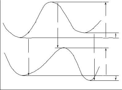
A compromise representation of our discussion thus far is to consider the effects of solvation on a one-dimensional slice through the energy surface –what we normally call the reaction coordinate –as illustrated in Figure 11.4. This representation is more informative than the free-energy cycle in showing how the structures of the stationary points differ in the gas phase and solution, in addition to their relative energies. A change in structure is indicated by a movement of the stationary point along the coordinate axis. Particularly for TS structures, which may be characterized by one or more soft normal modes and/or a soft reaction coordinate, changes in structure induced by solvation may be important.

Note, however, that this one-dimensional representation can be somewhat misleading if it is taken to be a computational protocol. The trouble is that the one-dimensional slice of

Arbitrary coordinate

Figure 11.4 Gas-phase (upper) and solution (lower) reaction coordinates, and the thermodynamic cycles that connect them via free energies of solvation of the various stationary points (vertical lines). Note the significant left to right movement of all stationary points, and particularly the TS structure, on going from the gas phase to solution