Cramer C.J. Essentials of Computational Chemistry Theories and Models

Choose basis set(s)

Optimize molecular geometry?

no

yes no

Does the current geometry satisfy the optimization

Output data for

criteria?

unoptimized geometry

yes

Output data for optimized geometry

Figure 8.1 Flow chart of the KS SCF procedure

orbitals are formed. In addition, the density itself may be expanded in an ‘auxiliary’ basis set. Such a concept may at first seem strange, since we know the density can be represented as the product of AO basis functions and density matrix elements, as it is in the Coulomb integrals of HF theory. However, in HF theory this is a natural choice because one needs to evaluate both Coulomb and exchange integrals, and in the latter the interchange of electronic coordinates requires that orbitals be used, not densities (which are the product of orbitals). In Eq. (8.21), however, there are no exchange integrals, so it is computationally convenient to represent ρ(r) with an auxiliary basis set, i.e.,

i=1

where the M basis functions have units of probability density (not the square root of probability density, as orbitals do) and the coefficients ci are determined by a least-square fitting to the density that is determined from the KS orbitals using Eq. (8.16). Note that the number of Coulomb integrals requiring evaluation in order to compute all the KS matrix elements in Eq. (8.21) is then formally N 2M, where N is the number of KS AO basis functions, instead of N 4, as is true for HF theory. As a result, the formal bottleneck in solving the KS SCF equations is matrix diagonalization, which scales as N 3, and one frequently sees in the literature reference to this reduced scaling behavior associated with DFT: compared to HF theory, DFT includes electron correlation and does so in a fashion that scales more favorably with respect to system size. However, many electronic structure programs do not employ auxiliary basis sets to represent the density, choosing instead to compute it in the HF-like way as a product of KS-orbital basis functions (the motivation for this choice was primarily historical: existing HF codes could be easily modified to carry out DFT calculations with this choice), in which case formal N 4 scaling is not reduced.

Continuing with our analysis of steps in the KS SCF procedure, after choice of molecular geometry, the overlap integrals and the kinetic-energy and nuclear-attraction integrals are computed. The latter two kinds of integrals are called ‘one-electron’ integrals in HF theory to distinguish them from the ‘two-electron’ Coulomb and exchange integrals. In KS theory, such an appellation is less clearly informative: all integrals can in some sense be regarded as one-electron integrals since every one reflects the interactions of each one electron with external potentials, but we will not dwell on the semantics. In any case, to evaluate the remaining integrals, we must guess an initial density, and this density can be constructed as a matrix entirely equivalent to the density matrix used in HF theory (Eq. (4.57)). With our guess density in hand, we can construct Vxc (and determine fitting coefficients for our auxiliary basis set if we are using the approach of Eq. (8.28)) and evaluate the remaining integrals in each KS matrix element. After this point, the KS and HF SCF schemes are essentially identical. New orbitals are determined from solution of the secular equation, the density is determined from those orbitals, and it is compared to the density from the preceding iteration. Once convergence of the SCF is achieved, the energy is computed by plugging the final density into Eq. (8.14) – this is in contrast to HF theory, where the energy is evaluated as the expectation value of the Hamiltonian operator acting on the HF Slater determinant. At this point either the calculation is finished, or, if geometry optimization is the goal, a determination of whether the structure corresponds to a stationary point is made.

Having reviewed the mechanics of the KS calculation, we now return to a discussion of how best to represent the exchange-correlation functional. We should be entirely clear on the nature of the LSDA approximation applied to a molecule. Invoking the uniform electron gas as the source of the energy expressions is not equivalent to assuming that the electron density of the molecule is a constant throughout space. Instead, it is an assumption that the exchange-correlation energy density at every position in space for the molecule is the same as it would be for the uniform electron gas having the same density as is found at that position.

8.4.2Density Gradient and Kinetic Energy Density Corrections

In a molecular system, the electron density is typically rather far from spatially uniform, so there is good reason to believe that the LDA approach will have limitations. One obvious way to improve the correlation functional is to make it depend not only on the local value of the density, but on the extent to which the density is locally changing, i.e., the gradient of the density. Such an approach was initially referred to as ‘non-local’ DFT because the Taylor-expansion-like formalism implies reliance on values of the density at more than a single position. Mathematically speaking, however, the first derivative of a function at a single position is a local property, so the more common term in modern nomenclature for functionals that depend on both the density and the gradient of the density is ‘gradientcorrected’. Including a gradient correction defines the ‘generalized gradient approximation’ (GGA).

Most gradient corrected functionals are constructed with the correction being a term added to the LDA functional, i.e.,

Note that the dependence of the correction term is on the dimensionless reduced gradient, not the absolute gradient.

The first widely popular GGA exchange functional was developed by Becke. Usually abbreviated simply ‘B’, this functional adopts a mathematical form that has correct asymptotic behavior at long range for the energy density, and it further incorporates a single empirical parameter the value of which was optimized by fitting to the exactly known exchange energies of the six noble gas atoms He through Rn (Table 8.7 at the end of this chapter provides references and additional details for B as well as for a reasonably complete menagerie of other functionals developed to date, including all of those discussed below). Other exchange functionals similar to the Becke example in one way or another have appeared, including CAM, FT97, O, PW, mPW, and X, where X is a particular combination of B and PW found to give improved performance over either.

Alternative GGA exchange functionals have been developed based on rational function expansions of the reduced gradient. These functionals, which contain no empirically optimized parameters, include B86, LG, P, PBE, and mPBE.

With respect to correlation functionals, corrections to the correlation energy density following Eq. (8.29) include B88, P86, and PW91 (which uses a different expression than Eq. (8.27) for the LDA correlation energy density and contains no empirical parameters). Another popular GGA correlation functional, LYP, does not correct the LDA expression but instead computes the correlation energy in toto. It contains four empirical parameters fit to the helium atom. Of all of the correlation functionals discussed, it is the only one that provides an exact cancellation of the self-interaction error in one-electron systems.

Typically in the literature, a complete specification of the exchange and correlation functionals is accomplished by concatenating the two acronyms in that order. Thus, for instance, a BLYP calculation combines Becke’s GGA exchange with the GGA correlation functional of Lee, Yang, and Parr.

show that the exchange-correlation energy can then be computed as

1

Exc = (λ)|Vxc(λ)| (λ) dλ (8.31)

0

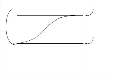
where λ describes the extent of interelectronic interaction, ranging from 0 (none) to 1 (exact). To evaluate this integral, it is helpful to adopt a geometric picture, as illustrated in Figure 8.2. We seek the area under the curve defined by the expectation value of Vxc. While we know very little about V and as functions of λ in general, we can evaluate the left endpoint of the curve. In the non-interacting limit, the only component of V is exchange (deriving from antisymmetry of the wave function). Moreover, as discussed in Section 8.3, the Slater determinant of KS orbitals is the exact wave function for the non-interacting Hamiltonian operator. Thus, the expectation value is the exact exchange for the non-interacting system, which can be computed just as it is in HF calculations except that the KS orbitals are used. The total area under the expectation value curve thus contains the rectangle having the curve’s left endpoint as its upper left corner, which has area ExHF. The remaining area is

Figure 8.2 Geometrical schematic for the evaluation of the integral in Eq. (8.31). The area under the curve is the sum of the areas of regions A and B. As region A is a rectangle, its area is trivially computed to be one times the expectation value of the HF exchange operator acting on the Slater determinantal wave function for the non-interacting system, (0). The area of region B is less easily determined. One simplification is to assume (i) that (1)|Vxc(1)| (1) is equal to the corresponding computed value from an approximate DFT calculation and (ii) that area B will be some characteristic fraction of the area of the rectangle having dotted lines for 2 sides (e.g., if the curve is well approximated by a line, clearly the characteristic fraction would be 0.5). Note that if the curve rises very steeply from its left endpoint, i.e., the value of z in Eq. (8.32) is very close to 1, then the adiabatic connection method is of limited value

some fraction z of the area corresponding to the rectangle sitting immediately on top of the first; the second rectangle has area (1)|Vxc(1)| (1) − ExHF. Unfortunately, not only do we not know z, we also do not know the expectation value of the fully interacting exchangecorrelation potential applied to the fully interacting wave function. However, we may regard z as an empirical constant to be optimized. In that case, we may as well approximate the unknown right endpoint, and a convenient approximation is the Exc computed directly by some choice of DFT functional. We see then that the total area under the expectation value curve can be written as

In practice, Eq. (8.32) is usually written using another variable, a, defined as 1 − z, providing

This analysis forms the basis of the so-called ‘adiabatic connection method’ (ACM), because it connects between the non-interacting and fully interacting states.

If we adopt the assumption that the expectation value curve in Figure 8.2 is a line, simple geometry allows us to determine that z = 0.5. Use of this value defines a so-called ‘half- and-half’ (H&H) method. Using LDA exchange-correlation, Becke showed that the H&H approach had an error of 6.5 kcal mol−1 over a subset of the G3 enthalpy of formation test set mentioned in Chapter 7. This compared quite favorably with the GGA method BPW91, which had an error of 5.7 kcal mol−1 over the same set.

One may in some sense regard the ACM approach as being similar in spirit to the KS SCF scheme. In the latter case, one does not know the exact kinetic energy as a function of the density, so one employs a scheme where a large portion of it is computed exactly (as the expectation value of the kinetic energy operator over the KS determinant) and worries later about the small remainder. So too, the ACM approach computes a large fraction of the total exchange-correlation energy, and then worries later about the difference between the total and the exact (HF) exchange.

Of course, if one is forced to estimate a constant like a, one might just as well choose a value that maximizes the utility of the method. And one may legitimately ask whether inclusion of additional empirical parameters results in sufficient improvement to make such inclusion worthwhile. Becke was the first to do this, developing the 3-parameter functional expression

where a, b, and c were optimized to 0.20, 0.72, and 0.81, respectively. The name of the functional, B3PW91, implies its use of a three-parameter scheme, as well as the GGA exchange and correlation functionals B and PW91, respectively (recall that the expression for the LSDA correlation energy in PW91 is different from eq. 8.27).

Subsequently, Stevens et al. modified this functional to use LYP instead of PW91. Because LYP is designed to compute the full correlation energy, and not a correction to LSDA, the

B3LYP model is defined by

where a, b, and c have the same values as in B3PW91. Of all modern functionals, B3LYP has proven the most popular to date. Its overall performance, as described in more detail in Section 8.6, is remarkably good, particularly insofar as the three parameters were not optimized! Such serendipity is rare in computational chemistry. The O3LYP functional is similar in character to B3LYP, with a = 0.1161, b = 0.9262 (multiplying O exchange instead of B exchange), and c = 0.8133. The two differ, however, in that B3LYP uses the VWN3 LSDA correlation functional while O3LYP uses the VWN5 version. The X3LYP functional also uses the form of Eq. (8.35), with a = 0.218, b = 0.709 (multiplying a combination of 76.5% B exchange and 23.5% PW exchange instead of pure B exchange), and c = 0.129.

Because they incorporate HF and DFT exchange, ACM methods are also called ‘hybrid’ methods. Some interest has developed in so-called ‘parameter-free’ hybrid methods, but this terminology must be regarded with some skepticism. Analysis of simple oneand twoelectron systems like H2 and H2+ make it clear that the correct amount of HF exchange to include in any hybrid model using a GGA functional cannot be a constant over all species (or even all geometries of a single species; see, for instance, Gritsenko, Schipper, and Baerends 1996). In any case, besides the B3 methods a number of one-parameter models, restricting themselves to adjusting the percentage of HF exchange included in the functional, have been proposed. These include B1PW91 and B1LYP (a = 0.25, b = (1 − a), c = 1 in Eqs. (8.34) and (8.35), respectively), B1B95, mPW1PW91, and PBE1PBE (sometimes called PBE0 because the parameter dictating the percentage contribution of HF exchange, 0.25, was not empirically optimized, but instead chosen based on perturbation theory arguments, thus there are ‘zero’ parameters). Overall, the performance of these functionals, as well as other ACM functionals listed in Table 8.7, tends to be fairly comparable to the B3 methods.

From a careful comparison of DFT densities to those generated from highly correlated wave functions, He et al. (2000) concluded that inclusion of HF exchange in a hybrid functional makes up for an underestimation by pure functionals of the importance of ionic terms in describing polar bonds. However, one may also adopt a less formal viewpoint of the hybrid methods. Experience indicates that GGA functionals have certain systematic errors. For instance, they tend to underestimate barrier heights to chemical reactions. Hartree–Fock theory, on the other hand, tends to overestimate barrier heights. To the extent that errors in total HF energies track with errors in HF exchange energy, one may regard the addition of HF exchange to ‘pure’ DFT results as something of a back-titration to accuracy. With this in mind, Lynch et al. have reoptimized the percent HF exchange in the mPW1PW91 model against a database of energies of activation and reaction for hydrogen-atom transfer reactions, referring to this model as MPW1K (‘K’ for ‘kinetics’). MPW1K increases the percentage HF contribution in the functional from the ‘default’ value of 25% to 42.8%; this increase in HF exchange leads to significantly improved performance over the chosen test set, although Boese, Martin, and Handy (2003) have noted that so high a fraction of HF exchange degrades the functionals performance for geometries and atomization energies. Zhao, Lynch, and Truhlar performed an equivalent optimization of percent HF exchange

A quick comparison of this equation with Eqs. (8.15) and (8.18) should make clear that this expression is indeed valid; its form is reminiscent of Eq. (4.39) insofar as the energy is expressed as a sum of orbital energies (the first term on the r.h.s.) corrected for doublecounting of electron–electron interactions (the next three terms on the r.h.s.). In addition the nuclear repulsion term, which is constant for a given geometry, is explicitly written here for reasons that will become clear shortly.

Consider now the possibility that we are interested in minimizing the energy of Eq. (8.36), but only subject to the shape of the KS orbitals, not to changing the density. That is, having picked a density, we optimize the orbitals by variational minimization of basis set coefficients, but we do not then recompute a new density from those orbitals (note that with a fixed density and geometry, all terms on the r.h.s. of Eq. (8.36) are constants except for the KS orbitals in the initial sum). Such a process is analogous to extended Huckel¨ theory in the sense that it is non-self-consistent, i.e., we solve a secular equation analogous to Eq. (4.21) a single time in order to derive our KS orbital basis set coefficients and then we are finished. This protocol defines the Harris functional approach, where the fixed density is usually chosen to be the sum of unperturbed atomic densities computed by whatever manner is deemed most appropriate. Energies from Harris functional calculations are obviously unlikely to be particularly good, but the orbitals may themselves be useful either for qualitative analysis in systems where charge transfer between atoms is small (e.g., in pure solid metals) or as very good starting-guess orbitals for a follow-on calculation at some self-consistent level of theory (e.g., HF or KS DFT); see Cullen (2004) for other applications of the Harris functional).

To speed this process up further for very large systems, one can make some further assumptions entirely analogous to those found in semiempirical MO theory. In particular, one may assume

where ε is the KS energy of the atomic orbital basis function (usually Slater-type orbitals) in the neutral atom (or one could use an experimental ionization potential to replace this number, in a semiempirical spirit), and the off-diagonal matrix elements depend only on the two atoms involved, A and B, and T is the kinetic-energy operator and veff is the effective potential deriving only from the electron densities and nuclei of atoms A and B. The offdiagonal matrix elements then depend only on interatomic separation and can be computed once and then either fit to analytic functions or interpolated from tabulations over various distances.

This same restriction of consideration to no more than pairwise interactions can be adopted for the remaining terms on the r.h.s. of Eq. (8.36), which are usually grouped together and referred to collectively as the repulsive energy Erep, so that this energy component is computed as

where, again, the pairwise terms can be computed once for every pair of atoms and then either fit to analytic functions or tabulated for future reference.

With these further simplifications, enormously large systems may be handled fairly easily to include geometry optimization. This non-self-consistent protocol defines DFTB.

The critical assumption of DFTB, however, is that the charge density of a composite system is well represented by the sum of the charge densities of its unperturbed constituent atoms. Clearly such a situation is inconsistent with the polarization that occurs in bonds between elements having significantly different electronegativities. To address such polarized systems, we consider a generalization of Eq. (8.36) that is valid to second order in the density fluctuation δρ(r) about the fixed density ρ0(r), namely

E[ρ0(r) + δρ(r)] = E[ρ0(r)]

(8.39)

In the spirit of DFTB, one may consider δρ(r) to be decomposable into atomic contributions according to

A

where q is used for the atomic contribution to emphasize the analogy to partial atomic charge. The second-order term in Eq. (8.39) may then be written as

If the atomic charge distributions are assumed to be spherically symmetric, the effective inverse distance γ is computed as

where η is an atomic hardness (formally the second derivative of the atomic energy with respect to a change from neutrality in charge; η is well approximated as (IP − EA)/2, where IP and EA are the atomic ionization potential and electron affinity, respectively) and a and b are Slater-type s orbitals on atoms A and B, respectively, in which case the electron-repulsion integral has an analytic solution. Once again this function, for which the off-diagonal terms depend on the distance between atoms A and B, may be approximated with a simpler analytic form or tabulated for all relevant atomic pairs.

The presence of the partial atomic charges in Eq. (8.41), however, poses the question of how they are to be computed. A popular choice is to compute them from Mulliken population analysis (see Section 9.1.3.2), in which case the partial atomic charges depend on the KS