

Patterson, Bailey - Solid State Physics Introduction to theory
.pdf54 2 Lattice Vibrations and Thermal Properties
Then make the change n′ → n′ + 1 in the dummy variable of summation. Because of periodic boundary conditions, no change is necessary in the limits of summation. We obtain
Mω2un+1 − ∑n′V (n′ − n)un′+1 = 0 . |
(2.38) |
Comparing (2.36) and (2.38) we see that if pun = 0, then pun+1 = 0. If pf = 0 had only one solution, then it follows that
un+1 = eiqaun , |
(2.39) |
where eiqa is some arbitrary constant K, that is, q = ln(K/ia). Equation (2.39) is an expression of a very important theorem by Bloch that we will have occasion to discuss in great detail later. The fact that we get all solutions by this assumption follows from the fact that if pf = 0 has N solutions, then N linearly independent linear combinations of solutions can always be constructed so that each satisfies an equation of the form (2.39) [75].
By applying (2.39) n times starting with n = 0 it is readily seen that
un = eiqnau0 . |
(2.40) |
If we wish to keep un finite as n → ± ∞, then it is evident that q must be real. Further, if there are N atoms, it is clear by periodic boundary conditions that un = u0, so that
qNa = 2πm , |
(2.41) |
where m is an integer.
Over a restricted range, each different value of m labels a different normal mode solution. We will show later that the modes corresponding to m and m + N are in fact the same mode. Therefore, all physically interesting modes are obtained by restricting m to be any N consecutive integers. A common such range is (supposing N to be even)
−(N / 2) +1 ≤ m ≤ N / 2 .
For this range of m, q is restricted to |
|
−π / a < q ≤π / a . |
(2.42) |
This range of q is called the first Brillouin zone.
Substituting (2.40) into (2.36) shows that (2.40) is indeed a solution, provided that ωq satisfies
Mωq2 = ∑n′V (n′ − n)eiqa(n′−n) , |
|
||||
or |
|
|
|
|
|
ωq2 = |
1 |
∑∞ |
V (l)eiqal , |
(2.43) |
|
M |
|||||
|
l=−∞ |
|
|
||

2.2 One-Dimensional Lattices (B) |
55 |
|
|
or
ωq2 = M1 ∑l∞=−∞V (l) cos(qla),
for an infinite crystal (otherwise the sum can run over appropriate limits specifying the crystal). In getting the dispersion relation (2.43), use has been made of (2.29).
Equation (2.43) directly shows one general property of the dispersion relation for lattice vibrations:
ω2 (−q) = ω2 (q) . |
(2.44) |
Another general property is obtained by expanding ω2(q) in a Taylor series:
ω2 (q) = ω2 (0) + (ω2 )′ |
q + |
1 |
(ω2 )′′ |
q2 + . |
(2.45) |
|
|||||
q=0 |
2 |
q=0 |
|
|
|
From (2.43), (2.33), and (2.34),
ω2 (0) ∑l V (l) = 0 .
From (2.44), ω2(q) is an even function of q and hence (ω2)′q=0 = 0. Thus for sufficiently small q,
ω2 (q) = (constant )q 2 or ω(q) = (constant )q . |
(2.46) |
Equation (2.46) is a dispersion relation for waves propagating without dispersion (that is, their group velocity dω/dq equals their phase velocity ω/q). This is the type of relation that is valid for vibrations in a continuum. It is not surprising that it is found here. The small q approximation is a low-frequency or long-wavelength approximation; hence the discrete nature of the lattice is unimportant.
That small q can be thought of as indicating a long-wavelength is perhaps not evident. q (which is often called the wave vector) can be given the interpretation of 2π/λ, where λ is a wavelength, This is easily seen from the fact that the amplitude of the vibration for the nth atom should equal the amplitude of vibration for the zeroth atom provided na = λ.
In that case
un = eiqnau0 = eiqλu0 = u0 ,
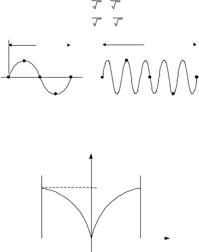
so that q = 2π/λ. This equation for q also indicates why there is no unique q to describe a vibration. In a discrete (not continuous) lattice there are several wavelengths that will describe the same physical vibration. The point is that in order to describe the vibrations, we have to know only the value of a function at a discrete set of points and we do not care what values it takes on in between. There are obviously many distinct functions that have the same value at many discrete points. The idea is illustrated in Fig. 2.2.

56 2 Lattice Vibrations and Thermal Properties
Restricting q = 2π/λ to the first Brillouin zone is equivalent to selecting the range of q to have as small a |q| or as large a wavelength as possible. Letting q become negative just means that the direction of propagation of the wave is reversed. In Fig. 2.2, (a) is a first Brillouin zone description of the wave, whereas
(b) is not.
It is worthwhile to get an explicit solution to this problem in the case where only nearest-neighbor forces are involved. This means that
V (l) = 0 (if l ≠ 0 or 1) .
By (2.29) and (2.34),
V (+l) = V (−l) .
By (2.33) and the nearest-neighbor assumption,
V (+l) +V (0) +V (−l) = 0 .
Thus
V (+l) = V (−l) = − |
1 |
V (0) . |
|||
|
|||||
|
|
|
2 |
|
|
By combining (2.47) with (2.43), we find that |
|||||
ω2 = |
V (0) |
(1 − cos qa) , |
|||
|
|||||
|
M |
|
|
|
|
or that |
|
|
|
|
|
ω = |
2V (0) |
sin qa . |
|||
|
M |
2 |
|||
(2.47)
(2.48)
This is the dispersion relation for our problem. The largest value that ω can have is
ωc = |
2V (0) . |
(2.49) |
|
M |
|
By (2.48) it is obvious that increasing q by 2π/a leaves the value of ω unchanged. By (2.35), (2.40), (2.41), and (2.48), the displacement of the nth atom in the mth normal mode is given by
(m) |
|
2πm |
||
xn |
= u0 exp ina |
|
||
Na |
||||
|
|
|
||
|
|
2V (0) |
||
exp it |
|
|||
M |
||||
|
|
|
||
|
|
a |
|
2πm |
|
|
|
||
|
|
|
|||||||
|
|
sin |
|
|
|
|
. |
(2.50) |
|
|
2 |
Na |
|
||||||
|
|
|
|
|
|
|
|
||
|
|
|
|
|
|
||||
This is also invariant to increasing q = 2πm/Na by 2π/a.
A plot of the dispersion relation (ω versus q) as given by (2.48) looks something like Fig. 2.3. In Fig. 2.3, we imagine N → ∞ so that the curve is defined by an almost continuous set of points.
2.2 One-Dimensional Lattices (B) |
57 |
|
|
For the two-atom case, the theory of small oscillations tells us that the normal coordinates (X1, X2) are found from the transformation
|
|
|
|
|
1 |
|
1 |
|
X |
1 |
|
|
2 |
|
2 |
|
|
|
= |
|
|||
|
X 2 |
|
|
1 |
− |
1 |
|
|
|
|
|
|
2 |
2 |
|
|
|
|
|
|
x |
|
(2.51) |
|
1 |
. |
|
|
x2 |
|
|
|
|
|
|
λ |
|
|
|
|
5λ |
|
|
|
|
|
|
|
|
|
|||
|
|
|
|
|
|
|
|
|
|
|
|
|
|
|
|
|
|
(a) |
(b) |
Fig. 2.2. Different wavelengths describe the same vibration in a discrete lattice. (The dots represent atoms. Their displacement is indicated by the distance of the dots from the horizontal axis.) (a) q = π/2a, (b) q = 5π/2a
ω


 ωc
ωc
|
|
q |
–π/a |
|
|
π/a |
||
Fig. 2.3. Frequency versus wave vector for a large one-dimensional crystal
If we label the various components of the eigenvectors (Ei) by adding a subscript, we find that
X i = ∑ j Eij x j . |
(2.52) |
58 2 Lattice Vibrations and Thermal Properties
The equations of motion of each Xi are harmonic oscillator equations of motion. The normal coordinate transformation reduced the two-atom problem to the problem of two decoupled harmonic oscillators.
We also want to investigate if the normal coordinate transformation reduces the N-atom problem to a set of N decoupled harmonic oscillators. The normal coordinates each vibrate with a time factor eiωt and so they must describe some sort of harmonic oscillators. However, it is useful for later purposes to demonstrate this explicitly.
By analogy with the two-atom case, we expect that the normal coordinates in the N-atom case are given by
X m′ = |
1 |
i2πm′n′ |
(2.53) |
||
N |
∑n′exp |
N |
xn′ , |
||
|
|
|
|
||
where 1/N 1/2 is a normalizing factor. This transformation can be inverted as follows:
1 |
|
− |
2πim′n |
|
N |
∑m′exp |
N |
X |
|
|
|
|
||
m′ |
= 1 |
∑ |
′ |
|
′ |
exp |
|
|
|
|
,n |
|
|||
|
|
N |
|
m |
|
||
|
|
|
|
|
|
|
|
|
= |
1 |
∑n′ xn′∑m′ |
||||
|
N |
||||||
|
|
|
|
|
|
|
|
2Nπi (n′ − n)m′ xn′
(2.54) exp 2Nπi (n′ − n)m′ .
In (2.54), the sum over m′ runs over any continuous range in m′ equivalent to one Brillouin zone. For convenience, this range can be chosen from 0 to N − 1. Then
|
|
|
|
|
|
|
|
2πi |
|
|
|
N |
||||
|
|
|
|
1− exp |
|
|
|
|
(n′− n) |
|||||||
N −1 |
2πi |
|
N |
|||||||||||||
|
|
|
|
|
|
|
|
|||||||||
∑m′=0 exp |
|
(n′− n)m′ |
= |
|
|
|
|
|
|
|
|
|
|
|
||
N |
|
1−exp |
2πi |
|
− n) |
|||||||||||
|
|
|
|
|
(n′ |
|||||||||||
|
|
|
|
|
|
|
|
|||||||||
|
|
|
|
|
|
|
|
|
|
|
|
|
||||
|
|
|
|
|
|
|
|
N |
|
|
|
|
||||
|
|
|
|
= |
|
|
1−1 |
|
|
|
|
|||||
|
|
|
|
|
−exp |
2πi |
(n′− n) |
|||||||||
|
|
|
|
1 |
||||||||||||
|
|
|
|
|
||||||||||||
|
|
|
|
|
|
|
N |
|
|
|
||||||
|
|
|
|
|
|
|
|
|
|
|||||||
|
|
|
|
= 0 |
unless n′ = n. |
|
|
|||||||||
If n′ = n, then ∑m′ just gives N. Therefore we can say in general that
1 |
∑N′−1 |
exp |
2πi |
(n′ − n)m′ |
= δ n . |
|
|
|
|||||
N |
m |
=0 |
|
N |
|
n′ |
|
|
|
|
|
||
Equations (2.54) and (2.55) together give
x |
|
= |
1 |
∑ |
|
|
− |
2πi |
|
′ , |
n |
N |
m′ |
exp |
N |
m′n X |
|||||
|
|
|
|
|
|
m |
which is the desired inversion of the transformation defined by (2.53).
(2.55)
(2.56)
2.2 One-Dimensional Lattices (B) |
59 |
|
|
We wish to show now that this normal coordinate transformation reduces the Hamiltonian for the N interacting atoms to a Hamiltonian representing a set of N decoupled harmonic oscillators. The reason for the emphasis on the Hamiltonian is that this is the important quantity to consider in nonrelativistic quantummechanical problems. This reduction not only shows that the ω are harmonic oscillator frequencies, but it gives an example of an N-body problem that can be exactly solved because it reduces to N one-body problems.
First, we must construct the Hamiltonian. If the Lagrangian L(qk , q·k , t) is expressed in terms of generalized coordinates qk and velocities q·k, then the canonically conjugate generalized momenta are defined by
pk = |
∂L(qk , qk ,t) |
. |
(2.57) |
|
∂qk |
||||
|
|
|
||
H is defined by |
|
|
|
|
H ( pk , qk ,t) = ∑ j q j p j − L(qk , qk ,t) . |
(2.58) |
|||
The equations of motion of the system can be obtained by Hamilton’s canonical equations,
qk |
= |
∂H |
|
, |
(2.59) |
|||
|
|
|||||||
|
|
|
∂p |
|
|
|
||
pk |
= − |
|
∂H |
. |
(2.60) |
|||
|
|
|||||||
|
|
|
|
∂qk |
|
|
|
|
If the constraints are independent of the time and if the potential V is independent of the velocity, then the Hamiltonian is just the total energy, T + V (T ≡ kinetic energy), and is constant. In this case we really do not need to use (2.58) to construct the Hamiltonian.
From the above, the Hamiltonian of our system is
H = |
M ∑n xn2 |
+ |
1 |
∑n,n′Vn,n′xn xn′ . |
(2.61) |
|
2 |
|
2 |
|
|
As yet, no conditions requiring xn to be real have been inserted in the normal coordinate definitions. Since the xn are real, the normal coordinates, defined by (2.56), must satisfy
X −m = X m . |
(2.62) |
Similarly x·n is real, and this implies that |
|
X −m = X m . |
(2.63) |

60 2 Lattice Vibrations and Thermal Properties
Substituting (2.56) into (2.61) yields
H = |
M ∑n |
1 |
∑m,m′exp − |
2πi |
n(m + m′) X m X m′ |
||||||
N |
|
||||||||||
|
2 |
|
|
|
N |
|
|
|
|||
+ |
1 |
∑n,n′Vn,n′∑m,m′ |
1 |
|
exp − |
2πi |
(nm |
+ n′m′) X m X m′. |
|||
2 |
N |
|
|||||||||
|
|
|
|
|
|
N |
|
||||
The last equation can be written
H= 2MN ∑m,m′ X m X m′∑n exp − 2Nπi n(m + m′)
+21N ∑m,m′ X m X m′∑n−n′V (n − n′)exp − 2Nπi (n − n′)m
×∑n′exp − 2Nπi n′(m + m′) .
Using the results of Problem 2.2, we can write (2.64) as
H = |
M |
∑m |
X |
|
X |
|
+ |
1 |
∑m |
X |
|
|
X |
−m ∑l |
V (l)exp |
− |
2πi |
lm |
|
, |
|||||||
|
m |
−m |
|
m |
|
|
|||||||||||||||||||||
|
2 |
|
|
|
|
|
|
2 |
|
|
|
|
|
|
|
|
|
|
|
|
|
|
|
N |
|
|
|
or by (2.43), (2.62), and (2.63), |
|
|
|
|
|
|
|
|
|
|
|
|
|
|
|
|
|
|
|
|
|
||||||
|
|
|
|
|
|
|
|
M |
|
2 |
|
+ |
1 |
|
2 |
|
X m |
|
2 |
|
|
|
|
|
|
||
|
|
|
|
|
|
|
|
|
|
|
|
|
|
|
|
|
|||||||||||
|
|
|
H = ∑m |
2 |
|
X m |
2 |
Mωm |
|
|
|
. |
|
|
|
|
|
||||||||||
|
|
|
|
|
|
|
|
|
|
|
|
|
|
|
|
|
|
|
|
|
|
|
|
|
|||
(2.64)
(2.65)
Equation (2.65) is practically the correct form. What is needed is an equation similar to (2.65) but with the X real. It is possible to find such an expression by making the following transformation: Define u and v so that
X m = um + ivm . |
(2.66) |
Since Xm* = X−m, it is seen that um = u−m and vm = −v−m. The second condition implies that v0 = 0, and also because Xm = Xm+N that vN/2 = 0 (we are assuming that N is even). Therefore the number of independent u and v is 1+2(N/2−1)+1=N, as it should be.
If the definitions z0 = u0
z1 = 2u1,…, z(N / 2)−1 = 2u(N / 2)−1, zN / 2 = uN / 2 , |
(2.67) |
z−1 =  2v1,…, z−(N / 2)+1 =
  2v(N / 2)−1
are made, then the z are real, there are N of them, and the Hamiltonian may be written, by (2.65), (2.66), and (2.67),
H = |
M |
∑mN=/ −2 |
(N / 2)+1(zm2 |
+ωm2 zm2 ) . |
(2.68) |
|
2 |
|
|
|
|

2.2 One-Dimensional Lattices (B) |
61 |
|
|
Equation (2.68) is explicitly the Hamiltonian for N uncoupled harmonic oscillators. This is what was to be proved. The allowed quantum-mechanical energies are then
E = ∑mN=/−2(N / 2)+1(Nm + |
1 |
) ωm . |
(2.69) |
2 |
By relabeling, the sum in (2.69) could just as well go from 0 to N − 1. The Nm are integers.
2.2.3 Specific Heat of Linear Lattice (B)
We will use the canonical ensemble to derive the specific heat of the onedimensional crystal.9 A good reference for the use of the canonical ensemble is Huang [11]. In a canonical ensemble calculation, we first calculate the partition function. The partition function and the Helmholtz free energy are related, and by use of this relation we can calculate all thermodynamic properties once the partition function is known.
If the allowed quantum-mechanical states of the system are labeled by EM, then the partition function Z is given by
Z = ∑M exp(− EM  kT ) .
If there are N atoms in the linear lattice, and if we are interested only in the harmonic approximation, then
E |
M |
= E |
m1,m2 |
,…,mn |
= ∑N |
m |
ω |
n |
+ |
|
∑N |
ω |
n |
, |
|
2 |
|||||||||||||||
|
|
n=1 |
n |
|
|
n=1 |
|
|
where the mn are integers. The partition function is then given by
|
|
|
|
|
|
|
|
|
|
|
Z = exp |
− |
|
∑nN=1ωn ∑(∞m ,m ,…,m |
|
)=0 exp |
− |
|
∑nN=1ωn mn . |
||
2kT |
N |
kT |
||||||||
|
|
|
1 2 |
|
|
|
||||
Equation (2.70) can be rewritten as
|
|
|
N |
N |
∞ |
|
|
|
|
|
Z = exp |
− |
|
∑n=1ωn ∏ ∑mn =0 exp |
− |
|
ωnmn . |
||||
2kT |
kT |
|||||||||
|
|
|
n=1 |
|
|
|
|
|||
(2.70)
(2.71)
9The discussion of 1D (and 2D) lattices is perhaps mainly of interest because it sets up a formalism that is useful in 3D. One can show that the mean square displacement of atoms in 1D (and 2D) diverges in the phonon approximation. Such lattices are apparently inherently unstable. Fortunately, the mean energy does not diverge, and so the calculation of it in 1D (and 2D) perhaps makes some sense. However, in view of the divergence, things are not as simple as implied in the text. Also see a related comment on the Mermin–Wagner theorem in Chap. 7 (Sect. 7.2.5 under Two Dimensional Structures).
62 2 Lattice Vibrations and Thermal Properties
The result (2.71) is a consequence of a general property. Whenever we have a set of independent systems, the partition function can be represented as a product of partition functions (one for each independent system). In our case, the independent systems are the independent harmonic oscillators that describe the normal modes of the lattice vibrations.
Since 1/(1 − α) = ∑∞0 αn if |α| < 1, we can write (2.71) as
|
|
|
N |
1 |
|
|
|
|
Z = exp |
− |
|
∑nN=1ωn ∏ |
|
|
|
. |
(2.72) |
2kT |
|
− exp(− ωn kT ) |
||||||
|
|
n=11 |
|
|
||||
The relation between the Helmholtz free energy F and the partition function Z is given by
|
|
|
|
F = −kT ln Z . |
|
|
|
|
|
|
|
||
Combining (2.72) and (2.73) we easily find |
|
|
|
|
|
|
|
|
|||||
|
|
|
|
|
|
|
|
|
ω |
||||
F = |
|
∑nN=1ωn + kT ∑nN=1ln 1 |
− exp |
− |
|
|
|
. |
|||||
2 |
kT |
|
|||||||||||
|
|
|
|
|
|
|
|
|
|
||||
Using the thermodynamic formulas for the entropy S, |
|
|
|
|
|
||||||||
|
|
|
|
S = −(∂F ∂T )V , |
|
|
|
|
|
|
|||
and the internal energy U, |
|
|
|
|
|
|
|
|
|
|
|||
|
|
|
|
U = F +TS , |
|
|
|
|
|
|
|
||
we easily find an expression for U, |
|
|
|
|
|
|
|
|
|||||
U = |
|
∑nN=1ωn + ∑nN=1 |
|
|
ωn |
|
|
|
. |
||||
2 |
exp( |
ω kT ) −1 |
|||||||||||
|
|
|
|
|
|
||||||||
(2.73)
(2.74)
(2.75)
(2.76)
(2.77)
Equation (2.77) without the zero-point energy can be arrived at by much more intuitive reasoning. In this formulation, the zero-point energy (ћ/2 ∑Nn=1 ωn) does not contribute anything to the specific heat anyway, so let us neglect it. Call each energy excitation of frequency ωn and energy ћωn a phonon. Assume that the phonons are bosons, which can be created and destroyed. We shall suppose that the chemical potential is zero so that the number of phonons is not conserved. In this situation, the mean number of phonons of energy ћωn (when the system has a temperature T) is given by 1/[exp(ћωn/kT − 1)]. Except for the zero-point energy, (2.77) now follows directly. Since (2.77) follows so easily, we might wonder if the use of the canonical ensemble is really worthwhile in this problem. In the first place, we need an argument for why phonons act like bosons of zero chemical potential. In the second place, if we had included higher-order terms (than the second-order terms) in the potential, then the phonons would interact and hence have an interaction energy. The canonical ensemble provides a straightforward method of including this interaction energy (for practical cases, approximations would be necessary). The simpler method does not.
2.2 One-Dimensional Lattices (B) |
63 |
|
|
The zero-point energy has zero temperature derivative, and so need not be considered for the specific heat. The indicated sum in (2.77) is easily done if N → ∞. Then the modes become infinitesimally close together, and the sum can be replaced by an integral. We can then write
U = 2∫ωc |
1 |
|
ωn(ω)dω , |
(2.78) |
|
exp( ω kT ) −1 |
|||||
0 |
|
|
|||
where n(ω)dω is the number of modes (with q > 0) between ω and ω + dω. The factor 2 arises from the fact that for every (q) mode there is a (−q) mode of the same frequency.
n(ω) is called the density of states and it can be evaluated from the appropriate dispersion relation, which is ωn = ωc |sin(πn/N)| for the nearest-neighbor approximation. To obtain the density of states, we differentiate the dispersion relation
dωn =πωc cos(πn / N ) d(n / N ), =  ωc2 −ωn2π d(n / N ) .
Therefore
Nd(n / N ) = (N /π)(ωc2 −ωn2 )−1/ 2 dωn ≡ n(ωn )dωn ,
or
n(ωn ) = (N /π)(ωc2 −ωn2 )−1/ 2 . |
(2.79) |
Combining (2.78), (2.79), and the definition of specific heat at constant volume, we have
Cv =
=
∂U∂T v
2N |
|
ω |
|
ω |
|
∫ |
|
||||
π |
|
c |
ω2 |
−ω |
|
0 |
|
||||
|
|
|
|
c |
|
|
|
ω |
|
−2 |
|
ω |
ω |
|
|
|
|||||||
exp |
|
−1 |
|
exp |
|
|
dω . |
|
2 |
kT |
|
|
kT kT 2 |
|
|||
|
|
|
|
|
|
|
|
|
In the high-temperature limit this gives
Cv = |
2Nk |
∫ |
ω |
|
2 |
−ω |
2 |
|
−1 |
2Nk |
sin |
−1 |
(ω /ωc ) |
ω |
c = Nk . |
π |
|
c |
ωc |
|
|
dω = |
π |
|
0 |
||||||
|
0 |
|
|
|
|
|
|
|
|
|
|
||||
(2.80)
(2.81)
Equation (2.81) is just a one-dimensional expression of the law of Dulong and Petit, which is also the classical limit.