Reactive Intermediate Chemistry

870 NANOSECOND LASER FLASH PHOTOLYSIS

5. CONCLUSION AND OUTLOOK

After 35 years, nLFPs has become a standard tool in photochemistry and physical organic chemistry. The choice of the right tools in terms of laser and detection systems, and a proper understanding to the kinetic methodologies available make it useful whether or not the intermediates of interest have a useful absorption in the spectral region accessible.

6. ACKNOWLEDGMENT

Thanks are due to the Natural Sciences and Engineering Research Council of Canada for generous support.

SUGGESTED READING

The reader is specifically referred to the following references: In addition, we recommend:

J.C. Scaiano, Ed., Handbook of Photochemistry, Vols. 1 and 2, CRC Press, Boca Raton, FL,

1989.

G.Bucher, J. C. Scaiano, and M. S. Platz, ‘‘Kinetics of Carbene Reactions in Solution,’’ in Radical Reaction Rates in Liquids, H., Fischer, Ed., Landolt-Bo¨rnstein, New Series II/18 Subvolume E2, Springer-Verlag, Berlin, 1998, Chapter 14, pp. 141–349.

REFERENCES

1.Nobel Prize presentation speech, 1967.

2.L. Lindqvist, Hebd. Seances Acad. Sci., Ser. C 1966, 263, 852.

3.G. Porter, ‘‘Flash Photolysis and Primary Processes in the Excited State,’’ in Fast Reactions and Primary Processes in Chemical Kinetics, Proc. 5th Nobel Symposium, S. Claesson, Ed., Almqvist and Wiksell, Stockholm, 1967, pp. 141–161.

4.R. D. Small, Jr., and J. C. Scaiano, J. Am. Chem. Soc. 1978, 100, 296.

5.M. S. Platz and V. M. Maloney, ‘‘Laser Flash Photolysis Studies of Triplet Carbenes,’’ in

Kinetics and Spectroscopy of Carbenes and Biradicals, M. S. Platz, Ed., Plenum Press, New York, 1990, p. 239.

6.R. A. Moss and N. J. Turro, ‘‘Laser Flash Photolysis Studies of Arylhalocarbenes,’’ in

Kinetics and Spectroscopy of Carbenes and Biradicals, M. S. Platz, Ed., Plenum Press, New York, 1990, p. 213.

7.R. A. McClelland, C. Chan, F. L. Cozens, A. Modro, and S. Steenken, Angew. Chem. Int. Ed. Engl. 1991, 30, 1337.

8.G. Cosa, L. Llauger, J. C. Scaiano, and M. A. Miranda, Org. Lett. 2002, 4, 3083.

9.J. A. Schmidt and E. F. Hilinski, Rev. Sci. Instrum. 1989, 60, 2902.

10.J. C. Scaiano, J. Am. Chem. Soc. 1980, 102, 7747.

REFERENCES 871

11.Luzchem Research, Inc. has developed a miniaturized laser system that takes advantage of these ceramic lamps: http :==www:luzchem:com.

12.J. C. Scaiano, J. Pineal Res. 1995, 19, 189.

13.M. V. Encinas, P. J. Wagner, and J. C. Scaiano, J. Am. Chem. Soc. 1980, 102, 1357.

14.R. D. Small, Jr., and J. C. Scaiano, Chem. Phys. Lett. 1977, 50.

15.H. Paul, R. D. Small, Jr., and J. C. Scaiano, J. Am. Chem. Soc. 1978, 100, 4520.

16.J. A. Howard and J. C. Scaiano, ‘‘Oxyl-, Peroxyl-, and Related Radicals,’’ in Rate and Equilibrium Constants for Reactions of Polyatomic Free Radicals, Biradicals and Radical Ions in Liquids, H. Fischer, Ed., Landolt-Bo¨rnstein, New Series II/13, Berlin, 1984, chapter 8.

17.R. D. Small, Jr., and J. C. Scaiano, Chem. Phys. Lett. 1977, 48, 354.

18.D. E. Falvey, Photochem. Photobiol. 1997, 65, 4.

19.S. E. Braslavsky and G. E. Heibel, Chem. Rev. 1992, 92, 1381.

20.R. V. Bensasson, E. J. Land, and T. G. Truscott, Flash Photolysis and Pulse Radiolysis; Pergamon Press, 1983.

21.I. Carmichael and G. L. Hug, J. Phys. Chem. Ref. Data 1986, 15, 1.

22.F. Wilkinson and G. Kelly, ‘‘Diffuse Reflectance Flash Photolysis,’’ in Handbook of Organic Photochemistry, Vol. I, J. C. Scaiano, Ed., CRC Press, Boca Raton, FL, 1989, pp. 293f.

23.J. C. Scaiano, L. J. Johnston, W. G. McGimpsey, and D. Weir, Acc. Chem. Res. 1988, 21, 22.

874 THE PICOSECOND REALM

1. OVERVIEW OF PICOSECOND-RESOLVED METHODS

The nanosecond and femtosecond realms are bridged by the picosecond regime not only in time but also in the level of complexity associated with the experiments. One must be prepared to evaluate critically the spectroscopic information that is obtained in the picosecond domain—more so than the nanosecond regime, but less so than the femtosecond time scale. Cautions will be noted and explained at appropriate times.

Think of a reactive intermediate that you want to study. Design a precursor that photochemically can produce your chosen intermediate. However, be careful! Chemical intuition should guide you in your preparation of a precursor. Previous reports of spectra for the reactive intermediate recorded in slower time domains or via matrix isolation should be used for comparison with picosecond spectra when attempting to make a firm assignment of a spectrum to a structure. If it is the first time that a spectrum has been assigned to a structure, use several chemically reasonable precursors in the experiments to learn if they all give the same— within experimental error—spectrum for the intermediate. There can be pitfalls. Unexpected chemical turns in the path from precursor to intermediate can lead to incorrect assignments. Beyond questions about chemistry lie important considerations about the specific spectroscopic technique that is employed in the investigation. While the picosecond realm differs less from the use of traditional spectrometers, such as an ultraviolet–visible (UV–vis) absorption spectrometer, than femtosecond-resolved methods, there are additional factors not considered in the nanosecond regime or with the use of continuous-wave spectrometers that can lead to the misinterpretation of data. It should be emphasized that the fundamental measurements need to be reproducible. The interpretations are subject to change as more information about a particular reactive intermediate is gathered.

In this chapter, we will look at several different picosecond-resolved spectroscopies and their applications to studies of organic reactive intermediates. Our focus will be on the use of time-resolved spectrometers whose first generated laser pulses have picosecond time durations. It is not meant to be an extensive review, but to provide examples of methods that are usable by organic chemists to study intermediates. These spectroscopic methods developed by chemical physicists have evolved to states that are welcome in the laboratories of physical organic chemists. Some of these methods may be more recognizable to organic chemists than others. However, the benefits of less common approaches will be described in sufficient detail to demonstrate the power of the broad range of laser-based systems that are currently in the arsenal of interrogating tools available for developing a greater mechanistic understanding of the roles of reactive intermediates in organic chemical reactions. The descriptions of the several systems herein are not intended to provide all the details, but enough of them to gain an appreciation of what is involved in the application of each spectroscopy covered in this chapter. Some of the pico- second-resolved spectroscopies, such as transient electronic absorption spectroscopy, have been established for quite some time whereas others have been developed more recently. Henceforth, any specific time-resolved spectroscopy

that probes the time regime from 1 to 999 ps will be referred to as a picosecond spectroscopy.

1.1. Ultraviolet–Visible Absorption Spectroscopy

One of the most commonly applied types of spectroscopy in the picosecond realm is pump–probe electronic absorption spectroscopy. The absorption spectra of reactive intermediates are usually just as featureless as those of the other two time domains described in this volume. It is simply the inherent nature of these spectra in condensed phases, most typically in solution. Spectroscopic studies in solution most closely mimic reaction conditions that reactive intermediates may find themselves involved in when they are formed and consumed during the course of an organic chemical reaction.

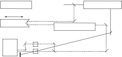
The key considerations of this experiment are the generation of the laser pulse of useful energy, the splitting of the pulse into the pump and the probe pulses, the conversion of the pump pulse into a wavelength suitable for excitation of the precursor to the reactive intermediate, the production of a probe pulse for interrogation of the evolution of the excited precursor, the timing of the arrival of the probe pulse relative to the pump pulse, and the measurement of how the intensity versus wavelength profile of the probe pulse changes as a function of the time that it passes through the sample relative to the excitation pulse (Fig. 19.1). The laser and detection systems may be of several types. Picosecond absorption spectrometers based on a solid-state laser and on a dye laser will be described.

variable

optical delay line conversion of primary ps pulse portion to probe pulse

reference

detector

beam sample splitter

Figure 19.1. Schematic diagram of a general pump–probe-detect laser spectrometer suitable for picosecond electronic absorption, infrared (IR) absorption, Raman, optical calorimetry, and dichroism measurements. For picosecond fluorescence—a pump-detect method, no probe pulse needs to be generated.

876 THE PICOSECOND REALM

1.1.1. Solid-State Laser Systems. The workhorse picosecond spectrometers are solid-state lasers and are based on an actively–passively mode-locked Nd:YAG oscillator, an yttrium aluminum garnet rod doped with neodymium(III) ions. What is described here is a typical spectrometer,1–3 but note that details may be different depending on the specific system that is under consideration. The Nd:YAG rod is pumped with microsecond-pulsed flashlamps at a rate of 10 Hz. Each flashlamp excitation produces a train of linearly polarized, 1064-nm pulses that are 30 ps at one-half maximum. A pulse selector, consisting of two crossed polarizers set on either side of a Pockels cell, senses the passage of a pulse located early in the pulse train and uses this pulse to trigger the Pockels cell to rotate the polarization of one of the more intense pulses in the train. This single, selected pulse is amplified in energy by passage through another optically pumped Nd:YAG rod—an amplifier— and then split into two pulses of approximately equal energy. Each of these two pulses needs to be amplified to sufficiently high energy to be converted from 1064 nm into 30-ps pulses to be used for excitation and interrogation of the sample.

A pulse suitable for excitation of an organic precursor to a reactive intermediate typically needs to be of a wavelength shorter than 1064 nm. To accomplish this without the use of a dye laser, which complicates matters relative to the use of a solid-state laser alone, other solid-state optical components—harmonic-generating crystals, also known as sum frequency generating crystals—are used to convert 1064-nm pulses into laser pulses of the second harmonic at 532 nm, to mix 532and 1064-nm pulses to generate the third harmonic at 355 nm, or to convert 532-nm second harmonic pulses into those of the fourth harmonic at 266 nm. These harmonics do not provide the broader excitation wavelength tunability exhibited via the use of a dye laser but do provide three wavelengths that have proved useful for a range of experiments. To achieve a greater palette of excitation wavelengths, one may use stimulated Raman scattering of the three harmonics, which involves the focusing of the selected, sufficiently energetic harmonic pulse through a Raman shifter—a cell fitted with entrance and exit windows and containing a gas under pressure. For example, if the gas were methane and the second harmonic were passed through the Raman shifter, 30-ps laser pulses shifted by the energy of the C H stretch to higher and lower energy from 532 nm along with residual 532 pulses can be selected through the use of filters or a prism and directed to the sample for excitation at a wavelength other than one of the harmonics. This is how the pump or excitation pulse is generated.

For picosecond, pump–probe transient absorption spectroscopy, the detector is not responsible for the time resolution. The recording of spectra as a function of time after sample excitation is achieved by optically delaying the arrival of the probe pulse relative to the pump pulse. These two pulses are born from a single, amplified 1064-nm pulse. If each one travels the same distance, corrected for delays induced as a result of passage through optical components, the pump and probe pulses will arrive at the sample at the same time. However, if the probe pulse travels a greater distance to reach the sample than the pump pulse, the probe pulse will interrogate the sample at a time after the pump pulse given by the distance–time relationship provided by the speed of light.

Before going further into the transient absorption experiment, let us turn our attention to the generation of the probe or interrogation pulse. One-half of the original 1064-nm pulse that is not used for making the pump pulse is focused into a cell that contains a 1:1 mixture of H2O and D2O to which 1% w/w P4O10 is added. An 30-ps, white-light continuum pulse, resulting from the nonlinear optical event of superbroadening of the 1064-nm pulse, exits the cell. For best continuum generation, 1064-nm pulses whose energies are in the range of 7–12 mJ are used. Competing with continuum generation is the occurrence of a longer time scale flash resulting from dielectric breakdown in the solution. It is important for the continuumgenerating solution to be as pure as possible and free from particulate matter. The former is accomplished through the use of high-quality H2O, D2O, and P4O10 while the latter can be insured by means of filtration through a membrane with 0.5-mm pores. Usable continuum intensity from 370 to 850 nm can be realized. The intensity versus wavelength profile of the continuum is shaped with filters so that the detector is not saturated for bands of wavelengths over the range of wavelengths that are monitored.

Now that we have the probe continuum and pump pulses generated, they are directed to the sample and the reference cells in a dual beam spectrometer configuration. The pump pulse is manipulated with reflectors and simple lenses. Prior to its passage through the sample cell, 8% is split from the pump pulse and sent to the probe of an energy meter so that pump pulse energies are monitored and can be maintained between 0.05 and 0.20 mJ/pulse. The continuum pulse is collected from the continuum generation cell with an achromatic lens that focuses it onto a pinhole covered with a diffuser. This pinhole target helps to separate the optics prior to continuum generation from the continuum direction optics. The image of the pinhole is magnified using an achromatic pair of lenses so that an 1.5-mm diameter spot exists at the sample cell and that the polychromator used to disperse the white-light continuum into a spectrum is suitably matched optically. The pump pulse spot is adjusted to be 1–2 mm in diameter.

The liquid sample is flowed through either a 1-, 2-, or 5-mm pathlength flow-cell at a rate sufficiently fast to replace the volume subjected to excitation by each pump pulse. Large sample volumes are used when possible to minimize the fraction converted to products. The sample solution is replaced when the product concentration becomes unacceptably high. If the sample emits light upon excitation, spatial filtering is used to maximize the rejection of the emission while permitting the confined diameter of the probe pulse to be collected optimally.

Prior to reaching the sample, the probe pulse is split into two pulses. One of the two is directed through the sample cell, and the other is passed through the reference cell. The reference cell is not flowed and contains sample solution that does not undergo excitation. The sample and reference probe pulses are dispersed and imaged onto two tracks of a multichannel detector. Types of detectors that are used include two-dimensional (2D) silicon intensified targets,1 double diode arrays,3–5 and charge-coupled devices (CCDs).6 Data collection and calculation of difference absorption spectra are performed with computer control. For the recording of a difference absorption spectrum, the probe pulse at a set optical delay

878 THE PICOSECOND REALM

relative to the pump pulse and the pump pulse are allowed to pass through the sample; one-half of the probe pulse is directed through the reference cell. The computer is used to collect and average the continuum intensity versus wavelength profiles that are transmitted through the sample and reference cells. This is done for a sufficient number of laser pulses to obtain an acceptable signal/noise ratio. Then shutters are closed via computer control to block the probe and pump pulses from the sample. For an amount of time equal to that of the previous acquisition of probe pulses, background is recorded and subtracted from the previously recorded probe pulses. After this, the same data-acquisition routine is followed except that the pump pulse is blocked from the sample. The absorbance change ( A) at a wavelength for a selected time postexcitation is given by Eq. 1.

The parameters Isðl; tÞ and Irðl; tÞ are the continuum intensities of the sample and reference tracks, respectively, when the sample is excited. The parameters I0sðl; tÞ and I0rðl; tÞ are the continuum intensities of the sample and reference tracks, respectively, when the sample is not excited. The continuum versus wavelength profile is dependent on the pulse energy used to generate it, and because it is a nonlinear optical phenomenon, changes markedly with relatively small changes in pulse energy. To correct for these changes, the ratio of I0rðl; tÞ=Irðl; tÞ is taken. Typically, 400 excitation–no excitation pairs are used to get good signal/noise ratios.

1.1.2. Dye Lasers. An example of a dye laser system used for transient absorption spectroscopy is that described by Wirz and co-workers.4 They based their system on the use of a dual-cavity excimer laser; one cavity is used to pump a cascade of dye lasers. At the core of the dye laser subsystem is a feedback dye laser that generates 0.5-ps, 496-nm pulses and whose output is amplified, frequency doubled (second harmonic generation), and used to seed a second, synchronously pumped cavity of the excimer laser. This process yields a 0.5-ps, 248-nm, 3.5-mJ pulse with a spot size of 1.5 cm2. The residual 0.5-ps, 496-nm pulse with an energy of180 mJ is used for the generation of the continuum pulse. The continuum pulse is collected with a spherical mirror, which is inherently achromatic, and the central portion containing the residual 496-nm pulse is blocked. The rest of the principles of the pump–probe transient absorption experiment are analogous to those described above for the Nd:YAG system. The dye laser in this instrument is not tuned to provide more excitation wavelengths. Additional details for the synchronously pumped dye laser spectrometer are given by Wirz and co-workers4 who also refer to a subpicosecond transient spectrometer described by Ernsting and Kaschke.5 This instrument used by Wirz and co-workers4 is noteworthy because its useful continuum spans from 310 to 700 nm. The ability to record spectra to shorter wavelengths is useful for studying organic reactive intermediates. However, one must keep in mind that dye laser systems are more challenging than solid-state

lasers to operate and to keep tuned during the course of recording a series of timeresolved absorption spectra.

Before moving to our next picosecond spectroscopy, there are three points of caution. First, be as confident as possible that the intensities of absorption bands change linearly with changes in pump pulse energy. This criterion does not insure that one-photon changes are induced upon excitation, however, because with the photon fluxes that can be generated with these lasers, the one-photon transition may be saturated and therefore give a linear response that reflects changes induced after the absorption of a second photon. Second, spectroscopists who use, without the recording of spectra, one of the harmonics, Raman-shifted, or a narrow band of the continuum to probe the kinetics of formation or decay of a reactive intermediate are cautioned in the interpretation of the data. This warning is particularly important in the study of the shorter end of tens of picoseconds after excitation. Without the benefit of viewing spectra, measurement of absorbance change for narrow wavelength bands can lead to conclusions about kinetics that are solely due to the shifting of the absorption band exhibited by an intermediate that is the result either of intramolecular vibrational relaxation or of stabilization via the reorientation of solvent molecules, and not a measure of the formation or decay of the reactive intermediate. The third path to incorrect interpretation of data is manifest at very short times after excitation, when the pump and probe pulses simultaneously occupy portions of the same space and therefore time. The generation of continuum, like any nonlinear optical process, gives rise to a pulse whose temporal profile is slightly less than the pulse used to generate it. Because the continuum spans a range of wavelengths, the shorter wavelength end is separated from the longer wavelengths through the effects of group velocity dispersion, commonly known as chirp. When chirp is not taken into account, an absorption that spans more than 100 nm and truly grows with a single time constant will appear to have its shorter wavelength end appear first, with the longer wavelength end appearing several or tens of picoseconds later depending on the width of wavelengths spanned by the absorption band. This problem arises when the continuum pulse is chirped after passing through optical components in which the shorter wavelengths travel more slowly than the longer wavelengths. At early times, the leading edge, richer in longer wavelengths, has already passed through the sample before the tailing portion of the continuum pulse, which is richer in longer wavelengths, overlaps with the leading edge of the pump pulse. Only the portion of the probe pulse richer in shorter wavelengths interrogates the excited volume of the sample, so only the shorter wavelength region of the time-resolved spectrum exhibits a positive absorption. The longer wavelength region of the spectrum lags in its increase in absorption as the probe pulse is moved to longer times after excitation that still overlap with the pump pulse. If the decay of this band is equally fast, the shorter wavelengths will appear to decay before the longer wavelength region of the absorption band decays. This artifact, resulting from the chromatography of light in the continuum pulse, will lead one to conclude that a shorter wavelength band feeds the longer wavelength band. If the decay of the shorter wavelength portion of the absorption band is not so fast, then one will erroneously conclude that there is a lag between

880 THE PICOSECOND REALM

the growth of the shorter wavelength portion relative to the longer wavelength portion when, in reality, both are appearing with the same rate constant.

1.2. Fluorescence Spectroscopy

Picosecond-resolved measurements of fluorescence intensities have been performed through the use of a streak camera1 and by means of time-correlated single photon counting (TCSPC)3. The former is a less instrumentationally involved approach provided that one has access to a streak camera. The TCSPC does allow a greater dynamic range for signal detection than streak camera measurements; however, the dynamic range for streak camera based detection has been a focus for improvement. Both of these approaches will be described here.

1.2.1.Streak Camera Detection. When a streak camera is used to measure the intensity versus time profiles of fluorescence in the picosecond regime,1,7 the com-

ponents that are used are based on those used for transient absorption described in Section 1.1, with the exception of the generation of a continuum probe pulse and the associated optics used for collecting reference and sample continuum light intensities. The streak camera coupled with a multichannel 2D detector capture the streak image of the fluorescence rise and decay. Both the quality of the streaking of the fluorescence with time and the correction of the response of the 2D detector over its area need to be known in order to obtain physically correct profiles of measured

light intensity versus time. The sample is flowed through an optical cell or a 3-mm diameter quartz tube and is excited with a pump pulse. At 90 to the path

of the excitation pulse, the fluorescence is collected with the use of an aspheric lens that can be precisely focused from the UV to the visible as needed for each specific sample.

A fluorescence event is recorded by splitting a portion of the 1064-nm pulse and directing it to a photodiode to trigger the electronics of the streak camera. The 1064-nm pulse is directed over a suitable distance to be used within the trigger window and converted to the wavelength desired for excitation of the sample. A portion of this excitation pulse is directed into the slit of the streak camera as a timing marker. The remainder of the pulse is passed to the sample. The light emitted from the sample can be filtered as needed to obtain information about the fluorescence behavior of the sample. The collected light is stored in a computer and treated with the time vector and 2D detector corrections. The rise times and decays are fitted in the usual manners that take into account the instrument response function.

1.2.2.Time-Correlated Single-Photon Counting. For the application of

TCSPC in the picosecond time domain, lasers with pulses whose half-widths are 20 ps or less are used.3 For better time resolution, the combination of a microchan-

nel plate photomultiplier tube (MCP-PMT) and a fast constant fraction discriminator (CFD) are used instead of a conventional photomultiplier tube (PMT). A TCSPC system with a time response as short as 40 ps has at its core a Nd:YLF (neodymium: yttrium lithium fluoride) laser generating 70-ps, 1053-nm pulses at