Molecular Heterogeneous Catalysis, Wiley (2006), 352729662X

436 Appendices

have been used to examine catalysis, however, have been performed at the MP2 level owing to the size and complexity of the systems modeled.

5.c. Couple Cluster Methods

Couple cluster methods di er from perturbation theory in that they include specific corrections to the wavefunction for a particular type to an infinite order. Couple cluster theory therefore must be truncated. The exponential series of functions that operate on the wavefunction can be written in terms of single, double and triple excited states in the determinant[2,14]. The lowest level of truncation is usually at double excitations since the single excitations do not extend the HF solution. The addition of singles along with doubles improves the solution (CCSD). Expansion out to the quadruple excitations has been performed but only for very small systems. Couple cluster theory can improve the accuracy for thermochemical calculations to within 1 kcal/mol. They scale, however, with increases in the number of basis functions (or electrons) as N 7. This makes calculations on anything over 10 atoms or transition-metal clusters prohibitive.

Returning to Fig. A8, there is a well-prescribed way of improving the accuracy for ab initio-based wavefunction calculations[2,14]. This involves an increase in the level of CI from:

HF < MP2 < CCSD < CCSD(T) < CCSDT(Q) Full CI

and also an increase in the relative extent of the basis set from:

single zeta (SZ) < double zeta (DZ) < double zeta with polarization (DZP) < triple zeta with double polarization (TZ2P)

Higher level CI calculations provide the most accurate predictions of properties including structures which can be determined to within 1%, reaction energies and enthalpies to within 1 kcal/mol, free energies to 2 kcal/mol and acid strengths to less than 2 pKa units.

This increase in accuracy, however, comes with a significant price in terms of CPU. Hartree–Fock formally scales as N 4 but most current methods can bring this down to N . The scaling for di erent CI methods, however, follows

MP2(N 5) < CISD, MP3 and CCSD(N 6) < MP4 and CCSD(T)(N 7).

The application of these methods has been limited in the area of catalysis since the sizes of the systems of interest are typically too big to handle at any level above MP2.

6. Density Functional Theory

6.a. Theory

The development of density functional theory (DFT) has had a tremendous impact on modeling heterogeneous catalytic systems. There are now a number of reviews which describe the application and impact of DFT on catalysis. The relative accuracy of DFT, along with the size of the systems that it can handle, makes it attractive for modeling heterogeneous catalytic systems[20−22,34]. Density functional theory is “ab initio” in the sense that it is derived from first-principles and does not require adjustable parameters. DFT methods formally scale as N3 and thus permit more realistic models of the intrinsic

438 Appendices

The Kohn–Sham equations are solved in a very similar manner to that used to solve the Hartree–Fock system in that one iterates on the correct spatial distribution of the electron density.

In the theory presented thus far, DFT can be considered as an exact approach. Unfortunately, the exchange correlation energy is not known. It is at this point where approximations must be introduced in order to solve the electronic structure problem.

The most basic solution to Eq. (A27) is to invoke the local density approximation which assumes that exchange-correlation per electron is equivalent to the exchange correlation per electron in a homogeneous electron gas which has the same electron density at a specific point r. This is typically written as:

EXC (r) = ρ(r)εXC ρ(r) dr (A31)

The local density approximation (LDA) is valid only in the region of slowly varying electron density. The LDA approximation is obviously an oversimplification of the actual density distribution and is well-known to lead to calculated bond and binding energies that are over-predicted[27] .

One of the primary shortcomings of the local density approximation is that the exchange correlation charge distribution is not spherically homogeneous. Non-local gradient corrections are introduced to allow for non-spherical electron density distributions [2,7,27]. As such, the correlation and exchange energies are functionals of both the density and the gradient with respect to the density. These gradient corrections take on various di erent functional forms which include the BP86 (Becke[28] and Perdew[29] corrections), PW91 (Perdew–Wang exchange functional)[30], PBE (Perdew–Burke–Ernzerhof)[31] or RPBE (Revised PBE functional)[32]. By way of example, the widely used Becke (B88) correction to the Local Spin Density Approximation to the exchange is given by

The functional takes on the correct r−1 asymptote behavior. xσ is the dimensionless density gradient shown in Eq. (A33) and ρσ is the density. The term b is simply a fitting parameter for the energy that is regressed against atomic data. Despite the importance of the exchange correlation functional, there is no formal path toward the development of more accurate functionals. The accuracy of DFT is therefore typically less than what can be expected from higher level ab initio methods such as coupled-cluster theory[2,5]. More recent developments in functionals attempt to couple an exchange component derived from Hartree–Fock theory which provides for a more exact match of the exchange energy for single determinant systems along with the correlation (and exchange) calculated from LDA theory in “hybrid” functionals. The most notable is the B3LYP functional, which is a combination of the Lee, Yang and Parr functional and the three-parameter model by Becke[33] :

EXB3LY P = a0HxHF + (1 − a0)ExLDA + axExB88 + (1 − ac)ECV W N + acEcLY P (A34)

Computational Methods 439

The theoretical chemistry community developed density functional theory for finite molecular systems which involve molecules and cluster models that describe the catalytic systems. They use the same constructs used in many ab initio wavefunction methods, i.e. Gaussian or Slater basis sets. The solid-state physics community, on the other hand, developed density functional theory to describe bulk solid-state systems and infinite surfaces by using a supercell approach along with periodic basis functions, i.e. plane waves[9] . Nearly all of our discussion has focused on finite molecular systems. In the next section we will describe in more detail infinite periodic systems.

6.b. Periodic Density Functional Theory Algorithms

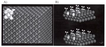
The cluster approach described so far can nicely begin to capture the local surface chemistry but is limited in terms of describing metals or metal oxides that take on more bulk-like characteristics including electronic, optical, and magnetic properties. In addition, there are also more practical considerations for solid-state periodic calculations which include the ability to examine readily surface relaxation and reconstruction e ects, higher surface coverages, and the degree of adsorbate ordering. The calculations for surfaces then are likely more easily modeled using a supercell approach along with plane wave basis functions[13]. The supercell is defined by three lattice vectors as well as the length along these vectors, thus providing a 3-D unit cell. The supercell is used to replicate the system infinitely along all three vectors using periodic boundary conditions, thus simulating the solid state. This is shown for the bulk structure of Pd in Fig. A9A. For three-dimensional bulk systems this is straightforward. The simulation of surfaces, however, requires that the metal atoms be truncated along the vector perpendicular to the surface and replaced with a vacuum region[13,21,34]. The unit cell is still repeated periodically along all three vectors. In this case, however, the result is a set of periodic slabs of some metal thickness sandwiched between two vacuum regions as shown in Fig. A9B.

Figure A9. Three-dimensional supercells used to replicate the bulk Pd metal and the Pd(111) surface

with adsorbed ethylidyne.

The wavefunction, according to Bloch’s theorem, is one which contains a wave-like portion [the exponential term in Eq. (A35)] and a periodic cell portion [the fi(r) term in Eq. (A35) and (A36)][13]. The wavefunction is expanded so as to take on the same periodicity of the lattice, where G defined in Gl = 2πm is the reciprocal lattice vector and m is an integer. The wavefunction is described by the summation of plane waves expanded out to a chosen cuto energy. k is the symmetry label in the first Brillouin zone.

440 Appendices

G

The choice of the cuto energy dictates the expansion of the wavefunction. Increasing the cuto energy is, therefore, similar to increasing the number of orbitals in a molecular calculation in that in increases the accuracy by allowing for more expansive wavefunction[13] The numerical integration for periodic solid-state systems is typically carried out in reciprocal space where the first Brillouin zone is divided and described by a finite number of k-points. The k-points describe the sampling of the electronic wavefunction. Observables such as the energy and the density are integrated over all k-points within the first Brillouin zone. Chadi–Cohen[35] and Monkhorst–Pack[36] are two particular approaches that have been developed to provide an optimal division of special k-points so as to provide a reasonably accurate description of the electronic potential. The total energy of the system should converge with increasing number of k-points since the increase in the number provides for a more dense k-point mesh and finer sampling of the Brillouin zone. The single particle wavefunctions are then described by plane wave basis sets that obey

Bloch’s theorem[13] .

Although plane waves are the natural choice for periodic systems, they pose di culties in accurately solving for the wavefunction near the core of the nuclei. The orbitals near the nuclei core are tightly bound and have significant oscillations, both of which make it di cult to model using expanded plane waves. They require an extensive number of plane waves, which is CPU intensive. Since most of the chemistry occurs via the valence electrons, the detailed electronic structure of the core can be avoided by using pseudopotentials. The pseudopotential approach, which was discussed earlier, substitutes the strong ionic potential and valence wavefunction with a weaker pseudopotential along with peudo wavefunctions. The pseudopotential removes the radial nodes in the core region and matches the valence electron wavefunction outside of the core region. This was shown in Fig. A5.

To summarize, the main di erences between the molecular and periodic DFT calculations involve:

1.the periodic replication of the unit cell which is described in a plane wave formalism as opposed to the local finite molecular system.

2.the basis set expansion is controlled by the cuto energy in the periodic system rather than by the number orbitals as it is in the molecular system.

3.the description of the system in reciprocal space verses real space for molecular systems.

Other than these di erences, the solution strategy is essentially the same for solving both the molecular and periodic systems.

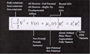
We have outlined here some of the main features in density functional theory. A number of other developments have occurred since its inception. Wimmer[6] elegantly captured some of the di erent approaches and how they di er with respect to the fundamental Kohn–Sham equations. An adaptation of one of his figures is give here in Fig. A10.

Computational Methods 441

Figure A10. A suite of options available in the solution of the Kohn–Sham equations for density functional theory. This figure nicely captures some of the essential di erences that exist between the full spectrum of di erent DFT codes that currently exists. Adapted from Wimmer [6].

7. Model Versus Method Accuracy

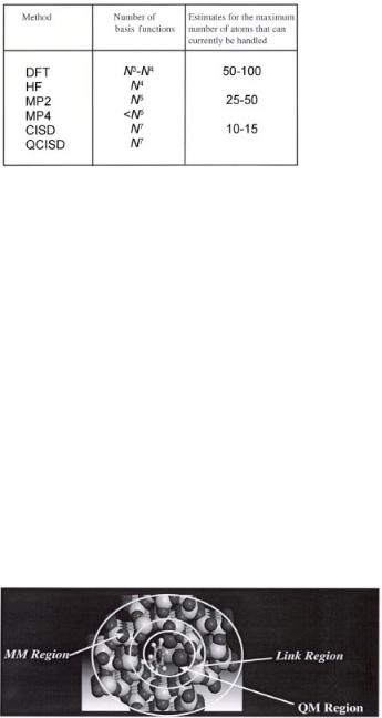
Method accuracy describes the relative accuracy of a quantum mechanical method based upon how well the quantum mechanical method can accurately predict electronic structure and energetics for an exact molecular structure or system[5,14]. In modeling heterogeneous catalytic systems, we seldomly can model all of the atoms in the system and must make a choice on how many atoms to include in the model of the active site and its environment. The size of the model used to describe the reaction environment can be critical to obtaining reliable numbers. While the calculations of small molecules such as NO, CO, ethylene, and NH3 on a single metal atom can be performed accurately by fairly using couple cluster theory, its relationship to the adsorption of these molecules on a metal surface is rather poor since a single metal atom cannot accurately represent the electronic structure of the metal surface. We describe this as the “model” accuracy as opposed to the method accuracy, which has been the focus to this point. In order to model catalytic systems, both the method and model accuracies need to be balanced. Most of the current e orts with heterogeneous catalytic systems have used density functional theory primarily to improve the model accuracy since DFT scales as N 3 and can thus allow the simulation of hundreds of atoms rather than 20 atoms or less. The scaling for some of the methods and the number of atoms that can be treated is shown in Fig. A11.

The relative accuracy of density functional theory methods for catalytic systems suggest, that the structures can typically be optimized to within 0.05 ˚Aand 1◦ in terms of bond lengths and angles, respectively[27] . Spectral properties such as infrared, Raman, and NMR can be predicted to within about 5% of the known experimental values. Optical properties which require excitation energies are less reliable for standard DFT methods. Time-dependent density functional theory, however, provides for a better estimation of

these properties. The binding energies and overall reaction energies from DFT methods are typically on the order of 5–8 kcal/mol in terms of accuracy[22,27,37]. This is not the

1 kcal/mol level of accuracy required for engineering purposes. In addition, there are also known outliers which are beyond the accuracy ranges cited. The accuracy of DFT methods is currently controlled by the exchange correlation energy functionals that are

442 Appendices

Figure A11. A comparison of the scaling and the approximate number of heavy atoms that can be handled by di erent theoretical treatments in the general order of increasing scaling and increasing accuracy. While the CISD and QCISD methods provide much more accuracy, the systems that can be examined are significantly smaller.

employed. These functionals, as discussed earlier, are somewhat arbitrary and therefore there is no systematic way of improving their accuracy. Despite these limitations, there is a wealth of current activity by various groups around the world towards the development of more accurate exchange correlation potentials.

8. Advancing to Larger Systems

There are various approaches that have been used to begin to simulate larger systems. The two most notable are the quantum-mechanical embedding and linear scaling methods.

8.a. (Quantum-Mechanical) Embedding

Quantum mechanical embedding involves dividing the reaction environment into di erent regions which are each treated using a di erent level of theory. The atoms directly connected to the actual reaction site are treated with a higher level of theory whereas those atoms which are further removed are treated with a lower level. The greatest di culty comes in linking two di erent regions together. The link region is usually defined in order to provide an adequate transfer of information between the inner and outer regions. The di erent regions are shown schematically in Fig. A12 for the adsorption site in a zeolite.

Figure A12. A schematic picture of the process of embedding for benzene adsorption at a metal oxide cluster fixed into the pore of a zeolite. The inner region which defines the adsorption site can be treated with a higher level of theory whereas the outer region is defined with a significantly lower level of theory such as force field. An overlap or “link” region is defined between the two in order to transfer information e ectively between the two models.

Computational Methods 443

The QM energy for this system is then calculated by the following equation:

where EQM(Core) refers to the QM energy calculated for the inner core region only. EMM(System) – EMM(Core) refers to the di erence in energy between the full system calculated using the lower level of theory and the core region using the lower level of theory. Although MM refers to molecular mechanics, it is not restricted to molecular mechanics. It can be any method which is a lower level method which is faster than the QM region of the core.

The ability to divide a system into separate regions and solve the inner system with a rigorous method and the outer region with a much faster method is fairly powerful. It allows for the simulation of systems comprised of O (104) atoms. In addition, it enables one to increase the accuracy of a particular calculation by using high-level CI calculations

to describe the central QM core region.

The earliest e orts in this area are ascribed to work by Warshel and Karplus[38]. It was not until the 1990s when it began to take on a much more active following. Perhaps the most widely used scheme is the ONIOM method, which was developed by Vreven

and Morokuma[5,39]. This is a general approach which is now part of the Gaussian suite of codes[123] . In the ONIOM method implemented into Gaussian, the user can choose

between various methods for both the core and exterior regions. Homogeneous catalytic systems, zeolites, and enzymes have all been modeled by using DFT or higher level quantum mechanical treatments for the core region and force field models to describe the external region. They can therefore capture the local reaction chemistry and also begin to describe the longer range e ects.

For supported metal and metal oxide systems, one typically has to resort to using two di erent QM methods owing to the lack of accurate force fields or empirical potentials to describe these systems. Both Whitten and Yang[40] and Govind et al.[41] have developed schemes which embed more accurate CI wavefunction methods into lower level QM methods in order to provide for more accurate descriptions than DFT. Sauer’s group has used

standard ab initio methods along with shell models to describe the oxide environment for zeolite systems[42,43].

8.b. Linear Scaling

A number of recent e orts have been focused on improving DFT’s N 3–N 4 scaling down to N . Linear scaling would thus enable one to examine much larger heterogeneous catalytic systems as well as biocatalytic systems. One of the inherent di culties in developing linear scaling methods resides in the Coulomb electron–electron repulsion integrals shown in Eq. (A38) which formally scale as N 4.

Very fast multipole methods have been developed in order to calculate these electron repulsion integrals[44,45]. The near field is determined by analytical Gaussian calculations. The far field is calculated using multipole expansions to treat the distant charges and their interactions. The scaling for this approach has been reduced to N 1.35. Fast quadrature

444 Appendices

methods for calculating the exchange correlation potentials have also been developed to improve scaling. In addition, there have been developments to provide linear-scaling approaches to the diagonalization of the density matrix. Traditional quantum mechanical methods are based on wavefunctions which characterize eigenstates for discrete energy levels. Orthogonality requirements on the wavefunction thus lead the system to scale as N 3. As the system grows larger, the wavefunction must extend over a much larger volume, thus increasing in larger basis sets[46] . In addition, more wavefunctions must be orthoganolized with respect to one another. These issues lead to N 3 scaling. The newer methods provide novel means of diagonalizing the density matrix to preserve linear scaling.

Siesta (the Spanish Initiative for Electronic Structure of Thousands of Atoms) is a self-consistent DFT method that demonstrates linear scaling for very large systems[47] . They do so by using flexible numerical atomic basis sets and localized linear occupations of orbitals. In addition, they project the electronic wavefunction and density onto real space grid in order to calculate Hartree and exchange correlation potential and matrix elements. The long-range features of the potential are eliminated by screening with local atomic electron density. Various other techniques are also employed to reduce the order dependence. Siesta has now been used to simulate various di erent systems. Simulation system sizes can begin to approach 10,000 atoms.

9. Ab Initio Molecular Dynamics

Classical molecular dynamics simulations have proven to be invaluable in determining the structure, sorption and di usion of organic molecules in various systems, including vapor, liquid, and mesoporous solid systems where accurate force fields and interatomic potentials have been derived. They fail, however, for systems which are not parameterized, including transition metals and transition metal oxides and sulfides. In addition, MD simulations can not be used to simulate chemical reactions or systems where electron transfer is important since the force fields are based on interatomic interactions with no treatment of the electronic structure. Simulating the dynamics of the electronic structure of a system requires the ability to follow the changes to the electronic structure as a function of time. Full quantum dynamic simulations present a significant challenge even for the simplest of systems. Fortunately, most systems obey the Born–Oppenheimer approximation, thus allowing us to separate out changes in the electronic and nuclear structure. As such, one can propagate the electronic structure with changes in the nuclear positions that result from molecular dynamics. In this way, one can do away with the necessity for an empirical force field. Instead, ab initio calculations are performed “on-the-fly” during the MD simulation to provide the forces on all of the atoms. These forces are then used to integrate the classical Newton’s equation of motion to find the new positions of the ions at the next point in time. In order to ensure accuracy, the time step used in the dynamics must be significantly shorter than that of the fastest processes. For bond making and breaking reactions, this is typically on the order of about 0.05 fs[48,55,57].

Ab initio molecular dynamics methods can roughly be divided into two classifications: Born–Oppenheimer Molecular Dynamics and Car–Parrinello Molecular Dynamics[55,56]. In both simulations, the wavefunction is propagated with the changes in the nuclear coordinates. In the Born–Oppenheimer MD approach, the forces on each of ions are explicitly calculated at each MD time step. As such, the system directly follows the Born– Oppenheimer surface. The primary drawback of the Born–Oppenheimer MD approach relates to the fact that time-intensive electronic structure calculations must be converged