Molecular Heterogeneous Catalysis, Wiley (2006), 352729662X

426 Appendices

atoms in order minimize the forces upon each atom and to converge upon the lowest energy of geometric structure for the system.

The initial atomic positions are necessary to describe the starting structure. The structure studied can be that of a simple molecule, a macromolecule, a bulk metal or metal oxide, the unit cell of a zeolite, a complex system comprised of catalytic surface along with adsorbates, solution molecules and ions, etc. Structures can be described in terms of Cartesian coordinates, direct coordinates, or z-coordinates[5] . The electronic structure can be mathematically represented by an infinite number of basis functions. More practically, these functions are truncated and described by a finite number of basis sets. A wide range of di erent basis sets currently exist and depend on the solution method used, the type of problem considered and the degree of accuracy required for solution. These functions can take on one of several forms, including Slater-type functions, Gaussian functions, and plane waves[6] . An infinite number of basis functions would be required for true accuracy and the complete electronic structure. This can be relaxed to a finite number of basis functions with some potential loss in accuracy. The number of basis functions used is then based on the relative degree of accuracy that one desires along with the CPU expenditures required to calculate.

The structural positions of the atoms and their basis functions are the only chemically specific input. Of course, there are typically a number of additional variables which describe the state of the system (the number of electrons, orbital occupations and the charge of the system), the type of calculation performed (a single point calculation, geometry optimization, a transition-state search, a molecular dynamics simulation), instructions on how the calculation is performed (the electronic and geometric convergence criterion, the density mixing scheme), the relative accuracy of the calculation (expanded basis sets, increased energy cuto s, etc.), and the specifications on output that are requested (orbitals, population analyses, density of states, frequencies, thermodynamic properties, etc.) that are all required.

2. The Potential Energy Surface

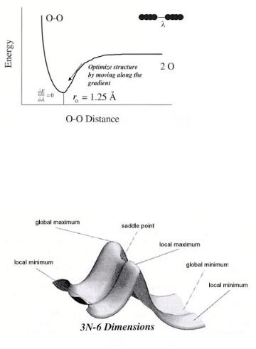
The output from the simulation of an optimized molecular structure includes the optimized atomic coordinates, which define the optimal structure, the optimized electronic structure for these specific coordinates and the total energy for this system. A schematic of the optimization of the O2 in the gas phase is shown in Fig. A2.

The energy for the O2 molecule is plotted at its initial starting geometry (i.e. λ= O–O distance = 2 ˚A) The electronic structure is calculated and subsequently used to determine the forces on each atom for the particular state that is being probed. These forces are then used to determine the new positions of the atoms in the system. This process is repeated in order to converge upon the energy for the optimized geometric structure. The results can be used to determine a host of di erent molecular properties, including electron density, electron a nity, ionization potential, relative energies for reaction processes, vibrational spectroscopy and a wide range of other chemical properties.

As we move from the one-dimensional O2 example shown in Fig. A2, the potential energy surface becomes much more complicated.

Figure A3, which was taken from Foresman and Frisch[5] , depicts the presence of local and global minima as well as local and global maxima. The local, and a global minima occur when the derivative of the energy with respect to the structural degree of freedom λi is zero for all degrees of freedom λi(dE/dλi = 0). Transition states occur at saddle points

Computational Methods 427

Figure A2. A schematic which shows the one-dimensional potential energy surface for O2 . The single defining internal coordinate, λi, is the distance between oxygen atoms. The energy is minimized when its derivative, with respect to changes in its Cartesian or its internal atomic coordinates, is zero (dE/dλi = 0) and the second derivative of energy, with respect to changes in its Cartesian or internal atomic coordinates, is greater than 0 (d2E/dλ2i > 0).

Figure A3. A more complex three-dimensional potential energy surface. The surface displays a global maximum and minimum (dE/dλi = 0) and transition (or saddle) points d2E/dλi 2 > 0 for all modes, λi, except the reaction trajectory, which instead is defined as d2E/dλi 2 < 0. The graph is reprinted from reference [10].

along the potential energy surface[2,4,5]. The derivative of the energy with respect to the degree of freedom λi is zero for all degrees of freedom for transition-state structures. In addition, the second derivative of the energy with respect to the degree of freedom λi is equal to zero for all degrees of freedom λi except for the mode which corresponds to the reaction coordinate.

3. General Electronic Structure Methods

Electronic structure methods can be categorized as ab initio wavefunction-based, ab initio density functional theoretical, or semiempirical methods. Wavefunction methods start

428 Appendices

with the Hartree–Fock (HF) solution and have a well-prescribed methods that can be used to increase its accuracy. One of the deficiencies of HF theory is that it does not treat electron correlation. Electron correlation is defined as the di erence in the energy between the HF solution and the lowest possible energy for the particular basis set that is used. Electron correlation refers to the fact that the electrons in a system correlate their motion so as to avoid one another. This physical picture then points out the deficiency of describing electrons in fixed orbital states. The electrons in reality should be further apart than predicted by HF theory. An exact solution of the Schr¨odinger equation requires the full treatment of electron correlation along with complete basis sets. Although this is unachievable, the breakdown of the inaccuracies into correlation and basis set expansion provides for a well-prescribed way in which to improve continually the accuracy and approach the exact wavefunction for the N -particle system.

Density functional theory is also derived from first principles but is fundamentally di erent in that it is not based on the wavefunction but instead on the electron density of the N -particle system[7] . Hohenberg and Kohn[8] showed that the energy for a system is a unique functional of its electron density. The true exchange-correlation functional necessary to provide the exact DFT solution, however, is unknown. The accuracy of density functional theory (DFT) is then limited to quality of the exchange-correlation functional that is used.

Semi-empirical methods avoid the solution of multicenter integrals that describe elec- tron–electron interactions and instead fit these interactions to match experimental data [4,9,10]. We will only discuss ab initio wavefunction and DFT methods here as they are more reliable for calculations concerning heterogeneous catalytic surfaces.

4. Ab Initio Wavefunction Methods

A series of general approximations are necessary in order to solve the Schr¨odinger equation. We have already introduced the Born–Oppenheimer and the time-independence approximations, which indicate that the energy of the system can be determined by solving for the electronic wavefunction.

4.a. Hartree–Fock Self Consistent Field Approximation

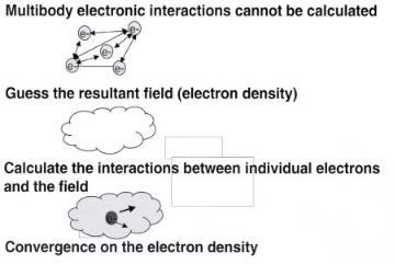
The self-consistent field approximation, which was briefly introduced earlier, is used to reduce the N -electron problem into the solution of n-single-electron systems. It reduces a 3n variable problem into n single electron functions that depend on three variables each. The individual electron–electron repulsive interactions shown in Eq. (A4) are replaced by the the repulsive interactions between individual electrons and an electronic field described by the spatially dependent electron density, ρ(r). This avoids trying to solve the di cult multicenter integrals that describe electron–electron interactions. The only trouble is that the electron density depends upon how each electron interacts with it. At the same time, the electron interaction with the field depends upon the density. A solution to this dilemma is to iterate upon the density until it convergences. The electron density that is used as the input to calculate the electron-field interactions must be equivalent, to within some tolerance, to that which results from the convergence of the electronic structure calculation. This is termed the self-consistent field (SCF).

This approach used in solving for n molecular orbitals within a self-consistent field is known as the Hartree–Fock solution[11,12]. The molecular orbitals are the individual electronic states that describe the spatial part of the molecular spin orbital[3]. Electrons are

430 Appendices

where Cij is a coe cient which relates the atomic orbital j to molecular orbital i. This is known as the basis set approximation[14]. More generally, the basis functions presented in Eq. (A8) do not have to be atomic orbitals but can simply be a series of basis functions used to describe the molecular orbitals. Atomic orbitals tend to be the most natural choice of basis functions for molecular-based systems. Gaussianor Slater-type basis functions are often used because they are easier to solve for computationally[2,4]. Solid-state systems described by periodic methods, on the other hand, are more naturally represented by using periodic plane wave basis functions[13]. In theory, the most accurate solution would require an infinite number of basis functions. Instead, the number of basis functions is truncated to a smaller set which is still able to capture the essential features of the wavefunction. The accuracy can improve by increasing the number and extent of the basis orbitals[14]. In the atomic basis scheme, for example, one can increase the number of basis functions on each atom to increase the size and spatial extent. In addition, polarization and di use functions can also be added to improve the displacement of electron density away from an atom in a particular environment as well as its spatial extent[2,4] . In periodic systems, the number of plane waves must be expanded[13] .

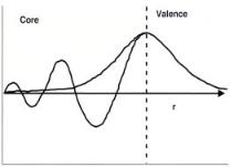
Full ab initio treatments for complex transition metal systems are di cult owing to the expense of accurately simulating all of the electronic states of the metal. Much of the chemistry that we are interested in, however, is localized around the valence band. The basis functions used to describe the core electronic states can thus be reduced in order to save on CPU time. The two approximations that are typically used to simplify the basis functions are the frozen core and the pseudopotential approximations. In the frozen core approximations, the electrons which reside in the core states are combined with the nuclei and frozen in the SCF. Only the valence states are optimized. The assumption here is that the chemistry predominantly takes place through interactions with the valence states. The pseudopotential approach is similar.

Figure A5. A schematic showing the comparison of the full electron wavefunction and the pseudopoten- tial-derived wave function. The strongly bound core electrons are replaced by a smoother analytical function. This schematic was adapted from Payne et al.13].

The valence electrons oscillate in the core region as is shown in Fig. A5, which is di cult to treat using plane wave basis functions. Since the core electrons are typically insensitive to the environment, they are replaced by a simpler smooth analytical function inside the core region. This core can also now include possible scalar relativistic e ects. Both the frozen core and pseudopotential approximations[13,15,16] can lead to significant reductions in the CPU requirements but one should always test the accuracy of such approximations.

Computational Methods 431

4.c. Hartree–Fock Solution Strategy

The single-electron wave equations from Eq. (A6) can be written in a more compact matrix form as the following equation:

where F t, Ct and S refer to the Fock, orbital coe cient and orbital overall intergral matrices, respectively. ε is a diagonal matrix which is comprised of the molecular orbital energies[5,16,17]. Hall[17] and Roothaan[18], simultaneously, proposed a solution strategy to solve the Hartree–Fock system based on the following secular equations:

ν=1

where Fµν refers to the Fock operator elements, Hµν are the Hamiltonian elements, Sµν are the overlap integrals for electrons in orbitals µ and ν, and Cνi are the molecular orbital coe cients. These matrix elements are defined by the following equations:

which more specifically refer to the Coulomb (Jij ) and exchange (Kij ) interaction between an electron and other electrons in the system.

The specific orbital energy levels can be written in terms of core Hamiltonian elements along with the Coulomb and exchange energies as follows:

432 Appendices

where P is the charge density matrix which is made up of the elements, Pλσ, which are comprised of the orbital coe cients Cλi and σi evaluated over all occupied orbitals:

The spatial electron density ρ(r) is defined by the density matrix elements as follows:

µ=1 ν=1

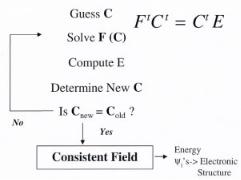
The solution strategy for solving for the self-consistent field and the final energy in the basic Hartree–Fock theory is shown in Fig. A6. The user starts with a simple guess for the initial ρ(r) density or the orbital coe cient matrix, C. The coe cient matrix can then be used to calculate the Fock elements. The Hamiltonian and overlap elements are also computed and used to solve the Roothan–Hall equations. This results in a new set of orbital coe cients along with the overall energy for the system. The new orbital coe cients are used to calculate new density and Fock matrix elements along with a new system energy. The procedure continues until the calculated density (orbital coe cients) is the same as that which was used in the input to the problem. The results ultimately provide the electron density, orbital overlap and the final energy state levels of the system.

Figure A6. Schematic illustration of the basic solution strategy for solving for the self–consistent field

and the final energy in Hartree–Fock methods.

For more in-depth discussions the reader is referred to texts by Jensen [2], Szabo and Ostlund[18] , Levine[3] , and Leach [4]

5. Advanced Ab Initio Methods

The Hartree–Fock solution strategy avoids the direct solution of electron–electron interactions but instead replaces these interactions by a mean field approach. This ignores the fact that the motion of individual electrons may be correlated. The schematic shown in Fig. A7 indicates that as the electron from point 1 moves toward point 2 , the electron

Computational Methods 433

at point 2 would likely move due to repulsive interactions between the two. The electrons therefore should have correlated motion. By definition, the di erence in the energy calculated by Hartree–Fock theory for a specific basis set which treats the systems as a mean field (without correlation) and the exact energy is the correlation energy. There are two primary strategies for treating correlated motion between electrons. Electrons with the same spin behave di erently to electrons with opposite spins. The basic Hartree–Fock theory already includes the treatment of electrons with the same spin by virtue of the fact that the wavefunction is required to be antisymmetric. Hartree–Fock theory, however, does not treat appropriately the interaction of electrons which have opposite spins. The wavefunction of the system, Ψ, cannot be described by a single determinant.

Three general approaches have been developed to treat electron correlation:

1.Configurational Interaction (CI),

2.Many Body Perturbation Theory

3.Couple Cluster (CC) theory.

The methods are briefly described below. More detailed discussions on each of these methods can be found elsewhere[2,14] .

Figure A7. A schematic cartoon illustrating the basic idea behind electron correlation. The movement or position of electron 1 should be correlated with the movement or position of electron 2 owing to the repulsive interactions that exist between the two.

5.a. CI Methods

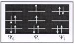
The general solution strategy for CI methods is to construct a trial wavefunction that is comprised of a linear combination of the groundstate wavefunction Ψ0 and excited-state wavefunctions Ψ1, Ψ2, etc. The trial wavefunction is shown in Eq. (A20), along with possible excited states Ψ1 and Ψ2:

The trial wavefunction can include the exchange of 1, 2 or 3 electrons from the valence band into unoccupied orbitals; these are known as CI singles (CIS), CI doubles (CID) and CI triples (CIT), respectively. CIS, CISD, and CISDT are methods configurational

434 Appendices

Scheme A1. Groundstate Ψ0 , single-excited state Ψ1 , double-excited state Ψ2

interaction methods which allow for single, single/double and single/double /triple excitations (see Scheme A1). All of these methods are based on the variational principle, which allows one to optimize the coe cients before each of the trial determinants shown in Eq. (A20). A full configurational interaction exchange (Full-CI) would involve all possible electron substitutions into the full manifold of occupied and unoccupied states. The Full-CI expression is Eq. (A21)

where CS , CD, and CT refer to the coe cients for the singly, doubly or triply excited states. The actual wavefunction now contains contributions from the ground state wave function Ψ0 and all of the other possible determinants. In addition to expanding the number of potential states, the coe cient multipliers for each state, Ci, can be optimized by variationally minimizing the energy. Full-CI calculations are computationallydemanding, and therefore, full-CI is possible only on very small systems. The multireference framework, however, provides a well-defined scheme for systematically improving the level of accuracy. Since these calculations are variationally optimized, the solutions should approach an accurate solution as the number of excitations increase. The full-CI then should begin to provide exact solutions within the limit of the basis set expansion. This will overcome the mean field approximation that is introduced in using Hartree–Fock.

All of the CI methods described so far are considered single determinant wavefunctions. Multiconfigurational SCF methods use multiple determinants[2,14]. In these methods, the coe ficients that multiply each state in Eq. (A21) and also the molecular orbital co- e cients used to construct the determinants must also be optimized. This involves an iterative SCF-like approach.

The second critical approximation that needs to be improved in order to improve accuracy is that of the limited basis functions used. Expanding the number of wavefunctions will help increase the resolution and accuracy. Figure A8 suggests that the most e cient improvement in accuracy come from increasing the CI treatment and basis set expansion together. The crudest HF basis set is that of a single valence. This can be improved by going to split valence, double valence, and triple valence along with adding polarization and di use functions. These increase the number of basis functions considerably, allowing for a more complete mathematical treatment of the wavefunction of the system.

Computational Methods 435

Figure A8. A comparison of model chemistries and their consistent improvement in accuracy as one increases both the correlation treatments and the completeness of the basis set. The optimal approaches for given CPU resources lie along the diagonal in that both the correlation and basis set are at optimal positions. Adapted from Head-Gordon [14] and Foresman and Frisch [5].

5.b. Many-Body Perturbation Theory/Møller–Plesset (MP) Perturbation

Theory

Many-body perturbation theory is based on the premise that the Hamiltonian from HF theory provides the basic foundation for the solution of the electronic structure and that configurational interactions can be treated as small perturbations to the Hamiltonian. The Hamiltonian is, therefore, written as the sum of the reference (HF) Hamiltonian (HO) and a small perturbation H :

where λ is a variable which describes the relative degree of perturbation. The perturbation is derived from the constructs of the true Hamiltonian and is equal to nuclear attraction and electron repulsion terms.

The wavefunction and the energy can then be written as a Taylor series expansion.

The terms E1, E2, E3, Ψ1, Ψ2, Ψ3, etc, are the higher order corrections to the energy and the wavefunction. The higher order corrections are solved subsequent to the unperturbed solution of Ψ0 and E0 from the H0 Hamiltonian.

The solution mechanism described is quite general. The most common choice for the reference of the unperturbed Hamiltonian operator is the sum over Fock operators. This is known explicitly as Møller–Plesset (MP) perturbation theory[2,19].

Most systems can be solved using relatively low perturbation orders, i.e. MP2 or MP4. MP2 can typically recover 80–90% of the correlation energy[2] . MP4 usually provides a reliably accurate solution to most systems. Nearly all of the studies where MP methods