Kosevich A.M. The crystal lattice (2ed., Wiley, 2005)(ISBN 3527405089)(342s)_PSa_

12.2 Quasi-Local Vibrations Near a Dislocation 283

The behavior of the function K0 (x) at small and large values of its argument is well known:

Thus, the vibration amplitude distant from the dislocation axis has a characteristic exponential decrease confirming that the vibrations are localized near the dislocation. The limiting dependence K0 (x) for x 1 shows that the vibration amplitude has a logarithmic singularity as ρ → 0. The equation (12.1.19) derived in the long-wave approximation is valid only for ρ a; therefore, the extremely small distance ρ for which (12.1.19) is valid may not be smaller than a.

12.2

Quasi-Local Vibrations Near a Dislocation

The equation for the eigenfrequencies (12.1.2) is equivalent to the condition

where G2(ε, k) is the Green function of the equation for 2D crystal vibrations (ε = ω2), with the spectrum of frequency squares (12.1.10) beginning with s2 k2, where k is a fixed parameter. This function has an obvious definition

G2 (ε, k) = ( a2)2 G0 (ε, k) d2k, 2π

where G0 (ε, k) is the Green function of an ideal crystal in a scalar model (4.5.10). The dislocation localized waves have frequencies for which Im G2 (ε, k) = 0. But

by examining quasi-local vibrations near a heavy impurity, we made it clear that in the frequency range where Im G2 = 0, resonance vibrational states may exist. In this case the frequencies of these vibrations are determined by

Using (12.1.12), it is easy to see that

It is clear that the r.h.s. of (12.2.3) tends to −∞ at the point ε = s2 k2 and determines the function symmetrical with respect to this point (Fig. 12.1). Finding from the plot a solution to (12.2.1), (12.2.2) we conclude that for Uk < 0 there are simultaneously solutions both to (12.2.1) for ε < s2 k2 (dislocation waves) and to (12.2.2) for ε > s2 k2 (quasi-local vibrations near the dislocation). But the latter have the physical meaning

284 12 Localization of Vibrations Near Extended Defects

Fig. 12.1 The real (1) and imaginary (2) parts of the Green function as functions of ε at fixed kz.

Fig. 12.2 The position of local ωd and quasi-local ωq frequencies of dislocational vibrations with fixed kz.

of isolated frequencies only in the case when the damping of a corresponding resonance frequency (i. e., the imaginary part of this frequency) is small. We know that the damping is determined by Im G2(ε, k) = π g(2)(ε, k), where g(2)(ε, k) is a twodimensional vibration density. In the considered range of frequency squares, π g(2) is

i. e., it has the order of magnitude of the square of a resonance frequency measured from the edge of the spectrum s2 k2. This means that the quasi-local frequency near a dislocation is very weakly pronounced.

In conclusion, we consider in brief a short qualitative characteristic of dislocation localized vibrations of a real crystal lattice that has three polarizations of the displacement vector with three branches of the dispersion law. In the isotropic approximation, there exist two branches of transverse vibrations with the dispersion law

12.3 Localization of Small Vibrations in the Elastic Field of a Screw Dislocation 285

ω2 = s2t (κ2 + k2 ) and one branch of longitudinal vibrations with the dispersion law

ω2 = s2l (κ2 + k2 ), so that sl > st always. If the value of k is fixed, there are two

bands of continuous frequency values of the bulk vibrations (Fig. 12.2) ω > sk. With the corresponding sign of the perturbation Uk, the frequency lying near the

boundary of the corresponding band may split off from the lower edge of each of the bands. One of these frequencies (the lowest one, ωd) corresponds to the vibration localized near the dislocation. It arises near the edge of the transverse vibration band and the localized vibrations have the form of transverse waves running along the dislocation. The dislocation axis participates in these vibrations, bending and vibrating like a spanned string. As the quantity stk − ωd is exponentially small, the bending waves have a velocity that practically does not differ from that of st. The character of vibrations allows us to formulate the elastic string model often used in different applications of a dynamic theory of dislocations. In this model a dislocation line is considered as a heavy string vibrating in a slip plane. The ratio of linear tension to dislocation mass is such that the dispersion law of string-bending vibrations coincides practically with the dispersion law of transverse sound waves in a crystal ω = stk.

The frequency “split off” from the boundary of the longitudinal vibrations spectrum (the frequency ωd in Fig. 12.2) could be considered as discrete only if the interaction between different branches of vibrations is disregarded. But the linear defect violates the independence of different types of vibrations so that they are “mixed together”. Since the frequency ωd2 is in the region of a continuous spectrum of transverse vibrations, it gets broadened and the corresponding vibration is transformed into a quasilocal one.

Finally, even in the case of an independent branch of vibrations, the quasi-local vibrations discussed in detail above are possible. These vibrations in Fig. 12.2 correspond to the frequencies ωq1 and ωq3 . The quasi-local peak width at the frequency ωq1 has been evaluated, and the peak width at ωq2 cannot be smaller. Hence, only the frequencies of bending vibrations of a dislocation as a spanned string are actually singled out.

12.3

Localization of Small Vibrations in the Elastic Field of a Screw Dislocation

The elastic vibrations near the dislocation as a source of static stresses in a crystal can be included, using a simple anharmonic approximation, into the initial state of a vibrating crystal and small vibrations on the background of a distorted lattice can be considered.

We represent the vibrating crystal displacement in the form

uz(ξ, z, t) = u0 (ξ) + u(ξ, z, t) ,

where u0 (ξ) is a static field of the screw dislocation coinciding with the axis Oz

286 12 Localization of Vibrations Near Extended Defects

((10.2.8) is convenient for this case)

u(ξ, z, t) are small dynamic displacements relative to a stationary crystal with a dislocation.

Apart from a static deformation, the equations of motion of a vibrating crystal with a dislocation will include anharmonicities (cubic and fourth-order ones). Then, restricting ourselves to the approximation linear in dynamic displacements, we get in a scalar model the following equation for the displacement u:

where λ and µ are the renormalized second-order elastic moduli taking into account anharmonicities (µ > 0, λ + 2µ > 0); A is the third-order elastic modulus; B and C are the fourth-order elastic moduli of a nonlinear elasticity theory (from general considerations, A B C µ).

Equation (12.3.2) should be supplemented with a certain boundary condition on the surface of a dislocation tube r = r0 to describe the phonon reflection from the dislocation axis. We use further the fact that no phonons penetrate into the region of the dislocation core. But we try, using the same approximation in which (12.3.2) is written to take correctly into account in the boundary conditions the symmetry of lattice distortions along the screw dislocation axis. If f (θ, z) is some function characterizing

that takes into account static displacements (12.3.1) about the screw dislocation. In view of (12.3.3), we write the solution (12.3.2) as

where m = 0, ±1, ±2, . . ..

It is typical that the solution (12.3.4) satisfying the screw symmetry (12.3.3) is nonperiodic with respect to the angle θ, and, therefore, is not a single-valued function of the coordinate x(ξ, z). We remember that u(x) is the atomic displacement relative to their equilibrium positions in a crystal with a dislocation, and x(ξ, z) are the atomic positions (coordinates) in a nondeformed crystal. The atom coordinates in a crystal with a dislocation, i. e., in a statically deformed medium, are different from those in

12.4 Frequency of Local Vibrations in the Presence of a Two-Dimensional (Planar) Defect 289

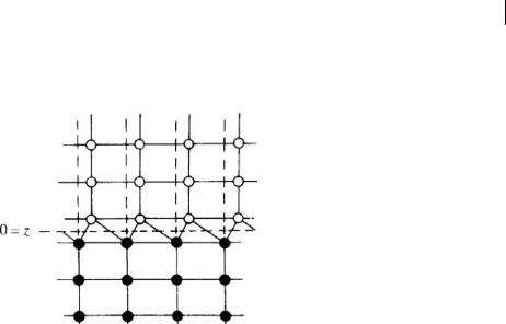
along the indicated surface (more frequently, it is a plane), the break in the rigorous lattice periodicity is called a stacking fault (Fig. 12.3). The possible types of planar stacking fault are completely determined by the crystallography of a given lattice.

Fig. 12.3 Planar stacking fault that is perpendicular to the z-axis.

We consider an unlimited, extended planar defect, assuming it to be coincident with a plane z = 0 parallel to some crystallographic plane. We restrict ourselves to the case of a symmetric lattice and assume that the z-axis is a four-fold symmetry axis of an ideal crystal. In general, the symmetry group of the plane defect is smaller than the corresponding group of atomic planes for an unbounded crystal lattice. Thus, there is no four-fold symmetry axis perpendicular to the defect plane in Fig. 12.3.

We show first that the equations of vibrations localized near such a defect coincide with the equations of vibrations of a certain 1D crystal. The stacking fault does not, generally, change the atomic mass; thus, it may seem that its influence on lattice vibrations is described only by the corresponding force matrix perturbations (just such perturbations are usually taken into consideration in qualitatively discussing the problem). However, if the interatomic distances in the stacking fault differ from those in a nondefect crystal lattice (h = a in Fig. 12.3) a local change in the mass density takes place. We intend to account for this fact.

The planar defect running through the whole crystal does not break the lattice homogeneity in a plane perpendicular to the z-axis. Then the perturbation potential U due to the change in the mass density along the defect layer can be written in the form analogous to (11.1.7)

where ∆ρ is the change in the mass density. Assuming such a form of the perturbation we unite two atomic layers (or crystallographic planes) on both sides of the plane z = 0 in Fig. 12.3 into one planar defect.

290 12 Localization of Vibrations Near Extended Defects

The perturbation of the force matrix U(n, n ) in this crystal should be dependent on the differences nx − nx and ny − ny and obey the requirement

Therefore, an equation of crystal vibrations including both types of perturbations is

ω2(n) − 1 ∑α(n − n )u(n ) m n

(12.4.2)

= ∑U(nx − nx, ny − ny; nznz)u(n ) + U0u(nx , ny, 0)δnz0 .

n

Since the crystal is structurally uniform in the x0y plane, it is convenient to switch in the equations of motion from a site representation in this plane to a two-dimensional k-representation, retaining the site representation along the the z-axis. We represent the amplitude of vibrations in the form

Uκ(nz, nz) = ∑ U(nx, ny; nz, nz)e−ia(kxnx +ky ny) .

nx ny

It is very important that the quantity κ appears in (12.4.3) as a parameter. If we assume this parameter to be fixed and are interested only in the dependence of the vibration amplitude on z, then omitting the index κ in all the quantities in (12.4.3), we obtain an equation for 1D crystal vibrations

where n = nz and the matrix V(n, n ) is equal

V(n, n ) = U(n, n ) + U0δn0δn 0.

The matrix Λ(n) has the following property ∑Λ(n) = ω02 (κ, 0), where the function ω0(κ, kz) determines the dispersion relation of an ideal crystal.

292 12 Localization of Vibrations Near Extended Defects

and use the ordinary Fourier expansion

In the approximation taken for calculations, the dispersion law of the crystal concerned is given by (12.4.5).

From (12.4.8), (12.4.9) we just find the dependence of the vibration amplitude on the coordinate z,

Setting z = 0 in (12.4.10), we find an equation for the possible frequencies of such vibrations

Before calculations of the integral in (12.4.11) look on the sketch of the vibration spectrum in Fig. 12.4. In Fig. 12.4. the hatched region corresponds to a band in the continuous spectrum of vibrations of an ideal crystal at small κ. The bottom ωlow(κ) and top ωup(κ) boundaries of this band are given by the expressions

Notations proposed in (12.4.12) allow us to give the simple representation of the calculation in (12.4.11):

Analyzing (12.4.12) and (12.4.13) we obtain localized states and their dispersion relations of the following types.

1. V0 > 0. In this case a frequency of the localized wave lies above the band of the continuous spectrum ω > ωup(κ) :