

Kosevich A.M. The crystal lattice (2ed., Wiley, 2005)(ISBN 3527405089)(342s)_PSa_
.pdf252 11 Localization of Vibrations
We substitute the result obtained in (11.1.17) and denote r = r(n)
1 |
|
|
r |
|
|
|
|
|
|
|
|
|
|
|
|||
Gε0 (n) |
|
exp |
− |
|
|
ω12 − ε . |
(11.1.18) |
|
r |
γ |
|||||||
Substituting (11.1.18) into (11.1.9) to obtain
u(n) = |
U0V0 u(0) |
exp − |
r |
, |
(11.1.19) |
||
4πγ2 |
|
r |
l |
||||
where the characteristic length l determining the localization region of vibrations with a discrete frequency is introduced:
l = |
√ |
γ |
= |
|
γ |
|
. |
(11.1.20) |
|
|
|
|
|
|
|||||
|
|
|
|
|
|||||
ε1 − εd |
|
ω2 |
− |
ω2 |
|||||
|
|
|
|
1 |
d |
|
|||
Thus, the local vibration amplitude decreases very quickly if the distance r increases and the decay length has the following order of magnitude
|
ω22 − ω12 |
|
ω22 − ω12 |
|
l a |
ω12 − ωd2 |
a |
δω |
, |
where ω2 − ω1 is the continuous spectrum frequency band width; δω = ω1 − ωd. Thus, the localization of vibrations is determined by the ratio of the gap size δω
separating a discrete frequency from the edge of the continuous spectrum to the width of the continuous spectrum band.
Note that local vibrations are concerned with many physical effects observed in crystals and indicate two aspects of this relation.
On the one hand, a discrete frequency separated by a finite range of frequencies from the continuous spectrum band results in singularities in the frequency dependencies of different characteristics of the scattering and absorption processes. Corresponding resonance singularities arise in the scattering amplitudes of different particles (e. g., neutrons) on local defects. Infrared absorption in ionic crystals also shows peaks corresponding to local vibrations of various centers specific to these crystals.
On the other hand, a local vibration has a finite weight in the expansion of the displacement vector of an impurity atom into normal modes of a defect lattice, unlike each mode of the continuous spectrum vibrations that has an infinitely small
weight (we remind ourselves that the contribution of a separate vibration of the quasi-
√
continuous spectrum is proportional to 1/ N, where N is the number of atoms in a crystal). Therefore, the effects connected with the displacement of impurity atoms and their nearest environment (e. g., optical transitions in impurity atoms, Mössbauer effect connected with impurity atoms, etc.) are very sensitive to local vibrations.

11.2 Elastic Wave Scattering by Point Defects 253
11.2
Elastic Wave Scattering by Point Defects
In general, the scattering problem can be subdivided into two parts: a calculation of the effective cross section for scattering and a study of the shape of the wave surface after scattering (at large distances from the scattering center). The first part of the problem requires knowledge of the local inhomogeneity structure (details of the point defect model). The second part concerns itself with the wave-surface shape at large distances and can be solved by very general assumptions concerning the character of the point defects.
A knowledge of the isofrequency surface shape is sufficient for studies of the asymptotic behavior of scattering waves. As we are interested in the scattering wave asymptotics, we restrict ourselves to the simplest model of a point defect, focusing on singularities of the isofrequency surface of a vibrating crystal.
The stationary vibrations of an ideal lattice are described by an equation represented symbolically by (2.2.2). The equation of crystal vibrations with an isolated defect is given in symbolic form by
1 |
|
εu − m Au = U u, ε = ω2, |
(11.2.1) |
where A is a linear Hermitian operator corresponding to the dynamic matrix of an
ideal crystal
Au(n) = ∑ A(n − n ) u(n ),
n
U is the perturbation matrix |
|
|
|
|
|
|
|
|
|
|
|
|
U u(n) = ∑U (n, n )u(n ). |
|
|
|
|
|
|
(11.2.2) |
|||||
n |
|
|
|
|
|
|
|
|
|
|
|
|
For an isotope defect positioned at the site n1 of a monatomic lattice, we have |
||||||||||||
Uik(n, n ) = U δ |
δ |
δ |
U = |
− |
ε |
∆m |
. |
(11.2.3) |
||||
|
||||||||||||
0 nn1 |
n n1 |
ik |
0 |
|
|
m |
|
|||||
We consider the scattering of the vibration mode of an ideal crystal |
|
|||||||||||
u(n, t) = u0 (n)e−iωt, |
|
u0 (n) = |
e(k0 ) |
eik0 r(n), |
(11.2.4) |
|||||||
|
√ |
|
|
|||||||||
|
N |
|||||||||||
by the point defect with a perturbation potential of the type (11.2.3) where we set n1 = 0.
Since the defect has no internal degrees of freedom, scattering will occur without change of frequency, and the coordinate part of the scattering wave is a solution to (11.2.1). We write the perturbed solution to this equation (in usual vector notations)
as |
|
u(n, t) = u0 (n) + χ(n), |
(11.2.5) |

254 11 Localization of Vibrations
where χ(n) describes the scattered wave and is a solution to the matrix equation (in the column notations)
1 |
χ = U (u0 + χ). |
|
ε − m A |
(11.2.6) |
A formal solution to this equation is found [similar to (11.1.9)] by using the Green
tensor of an ideal crystal (the index ε is omitted here) |
|
χ = G0U (u0 + χ). |
(11.2.7) |
Taking the noncommutativity of the operators in (11.2.7) into account we find that
χ = (1 − G0U )−1 G0U u0. |
(11.2.8) |
In the isotropic approximation or in a cubic crystal with only one isotope defect
producing the perturbation potential (11.2.3), the matrix G0U is diagonal, hence,
1 − G0U = 1 − Gε0(0)U.
Changing from the operator form of (11.2.8) to the coordinate form we find for the scattering wave (in the vector component notations)
i |
|
|
U0 |
ij |
|
j |
|
|
|
|
||
χ |
(n) = |
√ |
|
|
G0 |
(n)e |
(k0 ), |
|
(11.2.9) |
|||
ND(ε) |
|
|||||||||||
where |
|
|
|
|
|
|
∆m |
|
|
|
||
D(ε) = 1 − U0 Gε0(0) = 1 + |
ε |
Gε0 |
(0), |
(11.2.10) |
||||||||
m |
||||||||||||
and for a scalar model the r.h.s. of (11.2.10) should be understood literally, while for a cubic crystal G0(0) = (1/3)G0ll (0).
It follows from (11.2.9) that the form of a scattering wave at large distance is determined unambiguously by the asymptotic behavior of the Green tensor of an ideal lattice.
There is an expression (4.5.12) for the Green function in a scalar model. However, one can really use this formula for calculations only when (4.5.12) is rewritten in the form of an integral (4.5.13), but since the frequency ω is assumed to belong to the
eigenfrequency band of an ideal crystal, (4.5.13) should be regularized |
|
||||
|
V |
|
eikr(n)d3k |
|
|
Gε0 (n) = |
0 |
|
|
. |
(11.2.11) |
(2π)3 |
|
||||
|
|
ε − ω2(k) − iγ |
|
||
Regularization should result in a diverging wave at infinity, i. e., it should be the same as that used to determine the retarded Green function (Section 4.6).
Denote |
eikr(n)d3k |
|
|
|
I(r) = |
, |
(11.2.12) |
||
ε − ω2(k) − iγ |
and transform from an integration with respect to k to an integration with respect to z = ω2(k) and over the isofrequency surface z = const
I(r) = |
J(r, z) dz |
, |
(11.2.13) |
|
ε − z − iγ |
||||
|
|
|

11.2 Elastic Wave Scattering by Point Defects 255
where |
eikr(n) dSk |
|
|
|
J(r, z) = |
. |
(11.2.14) |
||
k ω2(k) |
||||
ω2(k)=z |
|
|
The main contribution to the asymptotic (at r → ∞) values of the integral (11.2.14) comes from the points of the stationary phase of the integrand. To elucidate the geometrical meaning of these points we write kr = rkn = rh (n is a unit vector in the direction r, and h = kn) and introduce the orthogonal curvilinear coordinate ξi (i = 1, 2) on the surface ω2(k) = z. The stationary phase points are then determined by the conditions
∂h |
= 0, |
i = 1, 2. |
(11.2.15) |
|
|||
∂ξi |
|
|
|
The conditions (11.2.15) are satisfied at the points where the supporting plane h ≡ kn = constant touches the isofrequency surface (Fig. 11.3a).
Fig. 11.3 Cross sections: (a) of an isofrequency surface on which the support points corresponding to the direction n are indicated; (b) of the wave surface on which the rays OS1 and OS2 limit the “folds”.
We denote the contact points by kν (sometimes they are called support points). On an isofrequency surface with an inversion center such points are positioned in pairs ±kν.
We consider one of the supporting points measuring the coordinates ξi from it. In the close vicinity of this point the following expansion holds:
h(ξ) = kνn + |
1 |
αikν |
|
αikν = |
∂2 h |
|
|
ξiξk, |
|
. |
|||
2 |
|
|||||
|
|
|
|
∂ξi ∂ξk ν |
||
We choose a network of curvilinear coordinates, so that the matrix ανik is diagonal, i. e., we choose the local coordinate axes ξ1 and ξ2 along the main directions of the surface curvature ω2 (k) = z at the point k = kν. Then
h(ξ) = kνn + |
1 |
α1ξ12 + α2ξ22 , α1 = α11, α2 = α22. (11.2.16) |
|
2 |
|||
|
|

256 11 Localization of Vibrations
With such a choice of 2D coordinates in k-space, the product α1 α2 determines the total (Gaussian) curvature of the surface at the tangent point; Kν = α1 α2. If Kν > 0, the corresponding point is called elliptical, and if Kν < 0 it is called hyperbolic.
All the points of a convex surface are elliptical. If the surface is not convex (such as shown in Fig. 4.3 or Fig. 11.3), there exist parts of the surface with points of different types (either elliptical or hyperbolic), but the parts of an isofrequency surface of the first and second types are divided by the lines along which one of the coefficients (α1 or α2) vanishes. These are the lines of parabolic points. Finally, at the intersection of the lines of parabolic points are the flat regions where α1 = α2 = 0.
We start by analyzing the asymptotic form of the integral (11.2.14) when the supporting points are elliptical or hyperbolic. Reducing the integral (11.2.14) to the sum of integrals in the vicinities of the tangent points (the points of the stationary phase),
we get |
|
|
|
|
|
|
|
|
|
|
|
|
|
|
|
|
|
|
|
|
|
|
J(r, z) = ∑ |
eikνr |
|
|
|
|
|
exp |
i |
r |
ξ12 + ξ22 dξ1 dξ2 |
. |
|
(11.2.17) |
|||||||||
2 |
|
|
|
|
|
|
|
|||||||||||||||
|
|
ν ω (kν) |
|
2 |
|
|
|
|
|
|
|
|
|
|
||||||||
|
|
|
|
|
|
|
|
|
|
|
|
|
|
|
|
|
||||||
The integrals in (11.2.17) are calculated simply to be |
|
|
|
|
||||||||||||||||||
|
|
|
|
|
|
∞ e±ix dx |
|
|
|
|
|
|
|
|
|
|||||||
|
i |
|
2 |
|
|
|
2π |
|
iπ |
|
|
|||||||||||
exp |
|
rαξ2 |
dξ = |
|
|
|
|
|
√ |
|
|
= |
|
|
exp |
± |
|
, |
(11.2.18) |
|||
2 |
|
r |α| |
|
|
r |α| |
4 |
||||||||||||||||
|
0 |
|
x |
|
||||||||||||||||||
where the sign in the exponent index coincides with the sign of the main curvature α. Thus we obtain an asymptotic expression proportional to 1/r (Lifshits, 1950)
|
|
|
exp |
ikνr ± |
|
iπ |
|
||
J(r, z) = |
2π |
∑ |
|
4 |
|
. |
(11.2.19) |
||
r |
2 |
(kν |
|
|
|
||||
|
ν |
|Knu| |
|
||||||
|
|
ω |
|
||||||
Substituting (11.2.19) into (11.2.13), we note that as r → ∞ the integral with respect to z is reduced to an integral over the close proximity of the point z = ε, where the integrand has a singularity. The main part of the integral (11.2.13) is obtained by integrating near the pole z = ε, so that the final asymptotic expression for the Green function (11.2.11) is
|
|
|
exp |
ikνr ± |
|
iπ |
|
|
|
|
Gε0(n) = |
iV0 |
∑ |
4 |
|
, |
(11.2.20) |
||||
4πr |
ω2(kν |
|
|
|
|
|||||
|
ν |
|
|Knu| |
|
||||||
where the summation is over |
the |
support |
points |
on |
the |
isofrequency surface |
||||
ω2(k) = 0 with nvν ≡ n ω(kν) > 0.
The asymptote (11.2.20) shows the necessary amount of decrease with distance ( 1/r), providing a finite value of the scattering wave energy flow in any finite interval of a solid angle dO. Indeed, the flow of the energy density of the elastic


258 11 Localization of Vibrations
expansion (Lifshits and Peresada, 1955): |
|
|
|
|
|
|
|
|
|
|
|
|
|
||||
|
√ |
|
|
4 |
|
|
|
|
|
|
|
|
iπ |
|
|
|
|
|
6πΓ |
|
|
exp |
ik0r ± |
|
|
|
|||||||||
J(r, z) = |
|
3 |
|
|
4 |
|
|
. |
(11.2.23) |
||||||||
5 |
|
|
|
|
2 |
|
|
|
1 |
|
|
1 |
|||||
|
|
r 6 |
|
|
|
ω |
(k0 ) |
|α| |
2 |
|β| |
3 |
|
|
||||
|
|
|
|
|
|
|
|
|
|
|
|
||||||
Calculating by means of (11.2.23) the asymptotes of the Green function and then the energy flow density, we find that the latter is proportional to r . If there are
no additional singularities on the line of parabolic points, then |α| |β| K where K is the Gaussian curve at an arbitrary point of the isofrequency surface. Thus, the
energy flow density along the direction n0 “catastrophically” exceeds at large r the energy flow density from the other points in the ratio r1/3 |β|1/6.
However, a solid angle inside which this energy flow density exists decreases with increasing r. Indeed, consider a scattered wave in the direction n inclined by an angle δθ2 (along ξ2) to n0 The supporting point will then be displaced by the value δξ2 determined by θ2 = 3β(δξ2 )2. In the new supporting point, the Gaussian curvature equals K = 6αβδξ2. Comparing with (11.2.19), where this Gaussian curvature is used with (11.2.23) for a parabolic supporting point, we see that they match by the order
of magnitude δξ |
|
|
( |
β |
| |
r)−1/3 |
. Thus, the angle inside which an increased energy |
||
|
2 |
| |
|
|
|
1/3 |
r−2/3. It is clear that the angle |
||
intensity is observed can be evaluated as δθ2 |β| |
|
||||||||
δθ2 decreases with increasing r faster than the energy density increases. Thus, the total energy flow per angle δθ2 decreases with distance proportional to r .
We ultimately calculate the contribution to the integral (11.2.14) generated by the flattening point in the vicinity of which an expansion of the function h is
h = k0 n0 + β1 ξ13 + β2ξ23.
Without repeating the calculations, we write down the corresponding part of the
integral (11.2.14) as |
|
|
|
|
|
|
|
|
|
|
|
|
3Γ2 |
|
4 |
|
|
|
|
eik0r |
|
|
|
J(r, z) = |
|
3 |
|
|
|
|
|
. |
|||
|
|
|
|
|
|
|
|||||
|
2 |
|
|
|
|
2 |
|
|
1 |
||
|
|
r 3 |
|
|
|
ω |
(k0 ) |
|β1 β2| |
3 |
|
|
|
|
|
|
|
|
|
|
|
|||
In the given case the energy flow density in the scattered wave exceeds that in the ordinary conditions in the ratio r2/3 |β1 β2 |−1/6 Accordingly, the solution of a solid
angle, where the flow of such density is concentrated, decreases with the distance as
|β1 β2 |1/3 r−4/3.
Having discussed the singularities of the scattered wave shape and its asymptotic behavior at infinity, we shall analyze in brief the frequency dependence of the scattered wave amplitude. The frequency dependence is primarily given by the multiplier D(ω2) in the denominator (11.2.9). The required regularization of this expression can
be performed using the relation (4.7.4) |
|
|
|
|
|
|
|
0 |
|
|
g0(z) dz |
|
|
||
D(ε) = 1 − U0 Gε−iγ |
= 1 − U0 |
P.V. |
|
|
|
− iπU0 g0(ε), |
(11.2.24) |
ε |
− |
z |
|||||
|
|
|
|
|
|
|
|


260 11 Localization of Vibrations
(11.1.6), i. e., it is found as a solution to the following equation vanishing at infinity
εGε − (A0 + U )Gε = I. |
(11.3.1) |
We rewrite (11.3.1) in the form (εI − A0 )Gε = I + U Gε and represent a formal
solution to this equation by means of the Green tensor of an ideal crystal G = G0 +
G0U G.
Performing calculations analogous to those used in deriving (11.2.8) we get
G = G0 + G0 T G0, |
(11.3.2) |
|
where the matrix T is determined by (11.3.2) |
|
|
T = I − U G0 −1 |
U . |
(11.3.3) |
In the present case of an isolated defect-isotope, T = [D(ε)]−1 U , where the definition (11.2.10) is used. Substituting (11.3.3) into (11.3.2) we obtain
Gik(n, n ) = Gik(n |
− |
n ) + |
U0 |
Gil (n |
− |
n |
)Glk(n |
1 − |
n ). |
(11.3.4) |
|
D(ε) |
|||||||||||
0 |
|
0 |
1 |
0 |
|
|
For a scalar model the formula (11.3.4) is not simplified much (only indices i, k, l are not used). The poles of the Green function as functions of the variable ε determine the squares of the eigenfrequencies of vibrations of the corresponding system (Section 4.5). It follows from (11.3.4) that the Green function for a crystal with a point defect may have an additional pole at the point where the function D(ε) is zero. Thus, the additional poles of the Green function (with respect to the ideal crystal Green function) determine the frequencies of local vibrations of a crystal with a defect considered in previous sections.
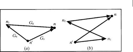
We shall now point out a specific structure of the Green function in a crystal with a single defect (11.3.4). By definition, the Green function concerned gives us a displacement of the n-th site in a lattice under the action of a unit force, which is periodic in time ω2 = ε and applied to the site n . In an ideal lattice, the stationary interaction is transmitted directly from the site n to the site n (the first term in (11.3.4)). In the presence of an isolated defect at the site n1 an additional excitation transfer channel through a defect appears (Fig. 11.4a) (this is the second term in (11.3.4)). In the second term the vector going to a defect or from it is associated with a multiplier G0, and the presence of the defect results in an additional multiplier U0/D(ε).
A remarkable feature of the excitation transfer through a defect possessing a local frequency is the resonance character of the transfer. By deriving (11.1.18) we have shown that the Green function Gε0 (n) decays exponentially with distance for the values of the parameter ε lying outside the band of the squares of the eigenfrequencies of an ideal crystal. Thus, at frequencies close to a discrete local frequency, the first term in (11.3.4) at large distances (r(n − n ) l) becomes negligibly small. The
11.3 Green Function for a Crystal with Point Defects 261
Fig. 11.4 Diagram for calculating the Green function in a crystal:
(a) with one impurity at the point n1 ; (b) with two impurities at the points n1 and n2 .
second term has a resonance denominator D(ε) and for ε can essentially exceed the first term. Thus, if the crystal has a defect with a discrete frequency in the forbidden band of frequencies of an ideal lattice, it promotes a resonance transfer of excitations at large distances. However, the second term in (11.3.4) also vanishes in the limit |n − n | → ∞ at any finite D(ε). The situation will be different if we go over from a crystal with one defect to a crystal with small, but finite concentration of defects.
Let us now see whether it is possible to use the method presented to find the Green function in a crystal with a system of point defects.
Unfortunately, the relation (11.2.22) between the matrix T and the matrix U is nonlinear, and the contributions of separate defects cannot be summarized in an equation such as (11.3.4). However, a solution generalizing (11.3.4) can also be found in this case.
We restrict ourselves to a scalar model and choose the perturbation matrix in the form
U(n, n ) = u0 ∑δnnα δn nα , |
(11.3.5) |
α |
|
where nα are the number vectors of the sites where the defects are positioned. For the matrix T one should expect a representation such as
T(n, n ) = ∑Tαβδnnα δn nβ . |
(11.3.6) |
αβ
Indeed, rewriting (11.3.3) in the form
(I − U Gε0)T = U ,
and substituting here (11.3.5), (11.3.6) we obtain a condition unambiguously determining a set of parameters Tαβ:
D(ε)Tαβ − U0 ∑ Gε0 (nα − ngamma)Tγβ = u0δαβ. |
(11.3.7) |
γ=α |
|