First, look at is the %util column to see what percentage of the disk is being used. As the example shows, the usage is low, which is expected because the machine is mostly idle. If values approach 100% here, that is a good indication of a disk bottleneck.

Next, look at svctm column, which lists the average number of milliseconds of time for the device to service an IO request. The lower the better, and anything over 7 or 8 starts to be a concern.

Also consider the avgqu-sz column metric, which reports the average queue length sent to the device. You typically want this to be in the single digits. Anything too low in conjunction with high disk usage can mean that the application is flushing to disk too often and not doing enough buffering, thus putting an extra load on the disk.

6.1.2 Tools available in InfoSphere CDC

InfoSphere CDC is the component that handles the replication of data between the solidDB front-end database and the back-end database. It is also a stand-alone product with many features that are not necessary in a solidDB Universal Cache configuration. Therefore, in this section we focus on the most useful and easy-to-use performance monitoring tools.

Management Console statistics

The GUI Management Console is capable of capturing replication statistics and presenting them in table and graph form. You must first enable statistics collection on your subscriptions first, as follows:

1.In the Subscriptions tab of the Monitoring view, right-click a subscription and select Show Statistics. A tab opens at the bottom half of the management console showing Latency, Source, and Throughput statistics tables.

2.Click Collect Statistics at the top left corner of this tab to enable statistics collection. The statistics tables and graphs are populated in real-time.

3.The graphs can be exported to Excel format by clicking Save Data at the top right corner of the statistics tab.

180 IBM solidDB: Delivering Data with Extreme Speed

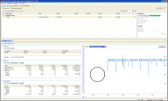
Figure 6-3 gives you an idea of the Management Console with a statistics view and a graph of Throughput Operations per second. This figure is from an active workload that was running in solidDB Universal Cache.

2,099

Figure 6-3 InfoSphere CDC Management Console Throughput Statistics

As Figure 6-3 shows, we were achieving 2,099 average operations per second. Our workload was not an exhaustive one so this number is by no means representative of the maximum operations per second that InfoSphere CDC is capable of replicating.

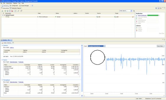
Figure 6-4 shows the same subscription and statistics view, except this time the live graph is showing log operations per second.

A number of live graphs are available to view the statistics.

2,112

Figure 6-4 InfoSphere CDC Management Console Log Operations Statistics

6.1.3 Performance troubleshooting from the application perspective

In this section, we address typical performance problems that might be encountered. It is structured to address typical perceived performance problems from the application’s perspective, such as the following problems:

Database response time (latency) is too high

Database throughput is too low

Database resource consumption is too high

Database performance degrades over time

Database response times are unpredictable

Special operations take too long

182 IBM solidDB: Delivering Data with Extreme Speed

Database response time (latency) is too high

Particularly for online transaction processing (OLTP) applications, database response time is a critical aspect of performance. The quicker SQL statements and transactions can run the better the results.

Ideally, an application has timing capabilities built into it to ensure statements and transactions are running fast enough to meet or exceed service level agreements. This usually means that the operations that are performed during that timing window are significantly more than simply reading the data from a table for example. Therefore, many possible causes for slow response time exist, and many possible cures are available. To fully realize where and how response time can be negatively affected, you should understand the steps that occur during the processing of a typical statement:

1.The function, for example SQLExecDirect(), is called by the application. Execution moves into the solidDB driver, but is still within the client application process. The driver builds a network message in a memory buffer consisting essentially of the SQL string and some session information.

2.The network message created by the driver is passed through the network to the solidDB server process. This is where network latencies can have a negative effect. Network messages can also be used within the same host machine also (local connections). solidDB supports a direct linking model called Accelerator and a shared memory access model (SMA), where the application contains all the server code also. Therefore, the following conditions are true:

–No need to copy the host language variables to a buffer

–No need to send the buffer in a network message

–No need to process the buffer in the server

–No context switches, that is, the query is processed within server code using the client application's thread context.

Using the Accelerator or SMA model essentially removes steps 1, 2, 5, 6 and 7 from the process.

3.The server process captures the network message and starts to process it. The message goes through the SQL Interpreter (which can be bypassed by using prepared statements) and the SQL Optimizer (which can be partly or fully bypassed by Optimizer hints). The solidDB server process can be configured to write an entry to tracing facilities with a millisecond-level timestamp at this point.

4.The query is directed to the appropriate storage engines (MME, disk-based engine, or both) where the latencies can consist of multiple elements:

–In the disk-based engine, the data can be found in the database cache. If it is, no disk head movements are required. If the data resides outside of cache, disk operations are needed before data can be accessed.

–in The main-memory engine, the data is always found in memory.

–Storage algorithms for the main memory engine and disk-based engine differ significantly and naturally have an impact on time spent in this stage.

–For complicated queries, the latency will be impacted by the optimizer decisions made in step 3, such as the choice of index, join order, sorting decisions, and so forth.

–For COMMIT operations (either executing COMMIT WORK or SQLTransEnd() by ODBC), a disk operation for the transaction log file is performed every time, unless transaction logging is turned off or relaxed logging is configured.

5.After statement execution is completed, a return message is created within the server process. For INSERT, DELETE, and UPDATE statements, the return message is always a single message that essentially contains success or failure information and a count of the number of rows affected. For SELECT statements, a result set is created inside the server to be retrieved in subsequent phases. Only the first two (configurable) rows are returned to the application in the first message. At this stage, an entry with a timestamp exists, written to the server-side soltrace.out file.

6.The network message created by the server is passed back to the driver through the network.

7.The driver captures the message, parses it and fills the appropriate return value variables before returning the function call back to driver application. The real response time calculation should end here.

8.Under strict definition, logical follow-up operations (for example retrieval of subsequent rows in result sets) should be considered as part of a separate latency measurement. In this chapter, however, we accept the situation where several ODBC function calls (for example SQLExecute() and loop of SQLFetch() calls) can be considered as a single operation for measurement.

Figure 6-5 on page 185 shows the eight steps of the statement processing flow. It suggests that latencies at the client depend on network response times and disk response times for all queries where disk activity is needed. Both response times are environment specific and cannot really be made much faster with any solidDB configuration changes. There are, however, ways to set up the solidDB architecture to prevent both network and disk access during regular usage.

184 IBM solidDB: Delivering Data with Extreme Speed

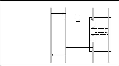
Reducing the database latency is essentially all about either reducing times spent within individual steps by design, architectural or configuration changes or possibly eliminating the steps altogether.

Figure 6-5 Statement processing flow

The importance of the steps depends fully on the type of load going through the steps. Optimization effort is not practical before the load is well understood. Consider the following two examples:

Example 1: The application tries to insert 1 million rows to a single table without indexes as fast as possible using prepared statements. Steps 1, 2, 3, 4, 5, 6, 7 are all small but they are executed a million times. An architectural change to use the directly linked accelerator or SMA model will help to bypass steps 1, 2, 5, 6, and 7, and will significantly speed up the operation.

Example 2: The application runs a join across 3 tables of 1 million rows each. The join returns 0 or few rows. Steps 1, 2, 5, 6, and 7 are executed only once and are trivial and fast. Steps 3 and 4 are executed once but are significantly more time consuming than they were in Example 1. Almost all the time will be spent in step 4, and removing steps 1, 2, 5, 6, and 7 does not bring meaningful benefits.

Optimization of simple write operation latencies

By simple write operations, we mean inserts, deletes, or updates to one table (preferably having few indexes) that modify only a small number of rows at a time. All the steps previously described are involved and none of the steps are extensively heavy.

The main performance issues are as follows:

If there is no need for persistence on disk for all operations, one of the following statements is true:

–There might not be a need to commit every time.

–Transaction logging could be turned off.

–Relaxed logging might be acceptable (perhaps in conjunction with HotStandby).

Simple write operations cause intensive messaging between client and server that can be optimized if use of the Accelerator linking or SMA model is possible.

In database write operations, finding the location of the row is generally a substantial part of the effort. solidDB's main memory technology enables faster finding of individual rows. Hence, using main memory technology can potentially improve performance with simple write operations. In most practical cases, it will be fully effective only after the need for disk writes at every commit has been removed one way or the other.

For small statements, running through the SQL interpreter is expensive. Hence, the use of prepared statements will improve performance.

In all write operations, all indexes must be updated also. The more indexes there are, the heavier the write operations will be. In complicated systems, there is a tendency to have indexes that are never used. The effort involved in validating whether or not all indexes are really necessary can pay off with better performance for write operations.

For simple write operation latencies, the effect of API selection (ODBC, JDBC, SA) is quite marginal. SA is the fastest in theory but the difference is typically less than 10%.

In theory, avoiding data type conversions (such as using DATE, TIME, TIMESTAMP, NUMERIC and DECIMAL) can improve performance. However, because of small number of rows affected, this effect is also marginal.

Key diagnostics in simple insertion operations

Many pmon counters can monitor overall throughput: SQL Execute, DBE Insert (or DBE Update, DBE Delete), Log file write, File write, Trans commit, and several HotStandby counters if HotStandby is being used. See “Performance Monitoring (pmon) counters” on page 148 for details about each counter.

For simple insertion latencies, Monitoring and SQL Tracing are the only available diagnostic tools within the solidDB product. See “Using the Monitor facility to monitor SQL statements” on page 163 for more details.

186 IBM solidDB: Delivering Data with Extreme Speed

Optimization of simple lookup latencies

In simple lookups, the database executes a query which is expected to return one row, or no rows at all. Also, index selection is considered to be trivial. That is, the where condition is expected to be directly resolvable by the primary key or one of the indexes.

Main memory technology was designed for applications running predominantly simple lookups. With these kinds of applications, performance improvements can be up to ten times better than databases using disk-based algorithms. If available RAM exists, using in-memory tables can be highly beneficial in these circumstances.

Similar to simple inserts, using prepared statements to avoid the SQL Interpreter being used for every statement execution and removing unnecessary network messages and context switches by using directly linked accelerator or SMA mode, can also improve performance.

Almost all discussions about database optimizers are related to bad optimizer decisions. With reasonably simple and optimized lookups in tables with several indexes, it is possible that the time used by the optimizer is substantial enough to be measurable. This time can be removed by using optimizer hints to avoid the optimization process altogether. See “Using optimizer hints” for more information.

Optimization of massive write operation latencies

Massive write operations differ from simple operations essentially by the number or rows being involved in a single operation. Both single update or delete statements affecting huge number of rows or a succession of insert statements executed consecutively are considered massive write operations in this section.

Massive write operations can conceptually have more of a throughput problem than a latency one however, we address them here mostly to aid in understanding and comparing these types of operations to others.

In solidDB’s disk-based tables, the primary key defines the physical order of the data in the disk blocks. In other words, the rows with consecutive primary key values reside next to each other (most likely in the same block) on the disk also. Therefore, by doing massive write operations in primary key order can dramatically reduce disk operations. With disk-based tables this factor is usually the strongest one affecting primary key design.

For example, consider a situation in which the disk block size is 16 KB and row size is 100 bytes, which means that 160 rows can fit in same block. We consider an insert operation where we add 1600 rows. If we can insert these 1600 rows in primary key order, the result is 10 disk block writes in the next checkpoint. If we are inserting the rows in random (with respect to the primary key) order, almost

all 1600 rows will access separate disk blocks. Instead of 10 file-write operations, the server could be doing 1600.

When running the massive write operations by executing a statement for every row (that is, not running update or delete that affect millions of rows), using prepared statements is important.

When running massive insertions with strict logging enabled, the size of the commit block is an important factor. If every row is committed, the disk head must be moved for every row. An optimal size for a transaction depends on many factors, such as table and index structures, balances between CPU and disk speed. We suggest some iteration with real hardware and data. Common starting values with typical applications and hardware would be in the range of

2000 - 20000. Fortunately, the performance curve regarding medium level transaction size is reasonably flat. The key is to avoid extremes.

For maximum performance of massive insertions in the client/server model, the solidDB SA API using array insert can have an edge over ODBC or JDBC. This way is mostly based on providing the programmer full control on inserting multiple rows in the same network message. solidDB ODBC and JDBC drivers provide support for bulk operations as defined by the corresponding standards. The implementations, however, are built on calling individual statement executions for every row in the bulk.

Excessive growth of the solidDB Bonsai Tree is the single most common performance problem experienced with disk-based tables. The problem is caused by the database preparing to respond to all queries with data as it was when the transaction started. Because disk-based tables’ optimistic locking allows other connections to continue modifying the data, duplicate versions of modified rows are needed. If a transaction lasts infinitely long, the Bonsai Tree grows infinitely large. With massive insertions, the problem can be caused by having one idle transaction open for a long time. The problem is relatively easy to detect and fix by closing the external connection.

Key diagnostics in massive insertions

The key diagnostics to follow are the pmon counters DBE Insert, DBE Delete, DBE Update, Trans commit, SQL Execute, File Write, and Ind nomrg write.

Optimization of complicated query latencies

In certain applications, most queries are in the complicated query category. Essentially this statement means that something else is required in addition to simply retrieving the rows, such as the following examples:

Sorting the data

Grouping the data

Joining the data across multiple tables

188 IBM solidDB: Delivering Data with Extreme Speed

The more complicated the query is, the more potential execution plans there are available for the optimizer to choose from when running the query. For example, there are many, many potential ways to execute a join of 10 tables.

Query optimization is a field of expertise all its own. solidDB, like all other major RDBMS products, has an optimizer to decide on the execution plan, which is essentially based on estimates of the data. Experience with query optimization for any other product is almost directly applicable when analyzing solidDB query optimization. For applications running complicated queries, preparation for bad optimizer decisions is an important step in system design. Even with low failure rates (say one in ten million), the impact of bad optimizer decisions might well transform a sub-second query to a query that will run for several hours.

The problem with bad optimizer decisions is that they are data specific and superficially random. For the decision, the optimizer selects a subset of randomly selected data from the tables and creates an estimate on the number of rows involved based on the random set. By definition, the random sets are not always similar and it is possible that a random set is sufficiently unlike the real data so as to mislead the optimizer.

With the randomness of the process, fully resolving the problem during the development and testing process is practically impossible. The application needs the capability of detecting the problems when they occur in the production system. When doing so, consider the following examples:

Detecting unexpectedly long response times can be done fully on the application level or it can be done using solidDB diagnostics such as SQL Trace files or the admin command sqllist.

To validate how incorrect the optimizer decision is, the bad execution plan must be captured also by running the EXPLAIN PLAN diagnostic of the query when the performance is bad. Running the query when performance is good does not prove anything. Building a mechanism into an application, which automatically collects EXPLAIN PLAN diagnostics for long lasting queries is suggested, but may not be trivial.

Almost always, bad execution plans (and even more so, the disastrously bad ones) are combined with an excessive number of full table scans. We show an example in “Example: How to detect full table scans from pmon counters with disk-based tables” on page 190. It describes how to look for patterns in pmon counters to understand when a full table scan might be in progress even without collecting EXPLAIN PLAN output for all queries.

Key diagnostics related to complicated query latencies

Often, complicated and heavy queries are executed concurrently with massive amounts of other (usually well-behaving) load. Then, in addition to executing slowly, they interfere with the other load also. Identifying this situation is not straightforward without application diagnostics. Finding one individual long-lasting query among hundreds of thousands of fast queries usually requires time and effort.

Before starting the task of finding potentially heavy queries executing full table scans, assess whether the perceived problems are likely to be caused by individual heavy queries. There is no exact method for that, but pmon counters Cache Find, DBE Find, and File read can be used to detect exceptionally large low-level operations indicating full table scans. Suggestions for doing this are in “Example: How to detect full table scans from pmon counters with disk-based tables” on page 190.

For finding long lasting queries among a huge mass of well-behaving queries, the following methods are available:

Use the admin command sqllist to list all queries currently in the server's memory.

SQL tracing with time stamps (either admin command monitor on or admin command trace on sql produce a potentially very large file containing all SQL executions. Finding the long-lasting ones from the big file might be time consuming but it can be done. See the following sections for more information:

–“Using the Monitor facility to monitor SQL statements” on page 163

–“Using the SQL Trace Facility to trace SQL statements” on page 168

After the problematic queries have been found, the execution plan can be validated with the EXPLAIN PLAN utility. See “Statement execution plans” on page 170 for more information.

Example: How to detect full table scans from pmon counters with disk-based tables

In this example, we describe how to detect full table scans from pmon counters with disk-based tables. The pb_demo table has an index on column J but not on column K.

190 IBM solidDB: Delivering Data with Extreme Speed

As expected, the execution plans shown in Example 6-16 illustrates an index based search and a full table scan.

Example 6-16 Sample explain plans showing an index scan and a table scan

4 rows fetched. Time 0.03 seconds.

Also, as expected, indexed searching is faster, as shown in Example 6-17.

Example 6-17 Comparing index based search versus table scan based search

1 rows fetched. Time 0.02 seconds.

The pmon counters, also show a distinct pattern. In Example 6-18 the un-indexed search (with admin command pmon accounting for the second SQL Execute) was run during the first time slice (the left-most column of numbers), while the indexed search was run during the second last time slice of 31 (third column of numbers from the right). The execute during the last time slice of 13 seconds is the second execution of pmon admin command.

Example 6-18 pmon counters for indexed and un-indexed search

To find full-table scans, search for the number of SQL Executes being disproportionate to the numbers for File Read, Cache Find, B-Tree node search mismatch and B-tree read operations. We can see in this example that we are doing 643 Cache reads and 2064 Cache finds for 2 SQL Executes. Then a few minutes later we are doing 0 Cache reads and 101 Cache finds for 1 SQL Execute. This is good evidence of a table scan being done in the first execution.

Optimization of large result set latencies

Creating a large result or browsing through it within the server process set is not necessarily an extensively heavy operation. Transferring the data from the server process to the client application through the appropriate driver will, however, consume a significant amount of CPU resources and potentially lead to an exchange of large amount of network messages.

For large result sets, the easiest way to improve performance is to use the directly linked accelerator or SMA options. It removes the need for network messages, copying data from one buffer to another and context switches, almost entirely. There are also key diagnostics that can be used to analyze the latencies of large result sets. They are the pmon counters SQL fetch and SA fetch, as well as fetch termination in the soltrace.out file.

When processing large result sets, applications are always consuming some CPU to do something about the data just retrieved. To determine how much of

192 IBM solidDB: Delivering Data with Extreme Speed

the perceived performance problem is really caused by the database, we suggest the following approach:

In a client/server architecture, look at how much of the CPU is used by the server process and how much by the application.

In an accelerator or SMA model, it is occasionally suggested to re-link just to assess database server performance. Also, rerunning the same queries without any application data processing might be an option

The difference between a fully cached disk-based engine and in-memory tables in large result set retrieval is quite minimal. Theoretically, disk-based engines are actually slightly faster.

In large result sets the speed of data types becomes a factor, because the conversion needs to be done for every column in every row to be retrieved. Some data types (such as INTEGER, CHAR, and VARCHAR) require no conversion between the host language and binary format in the database others do (such as NUMERIC, DECIMAL, TIMESTAMP, and DATE).

Database throughput is too low

In some cases, all response times seem adequate but overall throughput is too low. Throughput is defined as the count of statement executions or transactions

per time unit. In these types of situations, there is always a bottleneck on one or more resource (typically CPU, disk, or network) or some type of lock situation blocking the execution. Often, somewhat unexpected application behavior has been misdiagnosed as a database throughput problem, although the application is basically not pushing the database to its limits. This application behavior can be either the application consuming all of the CPU for processing the data on the application side, for example, or having only application-level locks (or lack of user input) to limit the throughput of the database.

In this section, we focus on what can be done in the database to maximize throughput.

Essentially, database throughput is usually limited by the performance of the CPU, disk, or network throughput. If the limiting resource is already known, focus only on the following principles.

To optimize for CPU-use:

–Avoid full table scans with proper index design.

–With disk-based tables, optimize the IndexFile.BlockSize configuration parameter. Smaller block size tends to lead to less CPU usage with a price of slower checkpoints.

–Assess whether MME technology can be expected to have an advantage.

–Use prepared statements when possible.

–Optimize commit block size.

To optimize for minimal dependency on disk response times:

–Use main memory tables when possible.

–With disk-based tables, make sure your cache size is big enough (optimize the IndexFile.CacheSize configuration parameter).

–Check whether some compromises on data durability would be acceptable. Consider turning transaction logging off altogether or using relaxed logging mode. These choices can be more acceptable if the HotStandby feature is used or there are other data recovery mechanisms.

To optimize for the least dependency on network messages:

–Optimize message filling with configuration parameters.

–Consider API selection (especially for mass insertion).

–Consider whether the volume of moved data can be reduced, for example by not always moving all columns.

–Consider architectural changes (for example, move some functionality either to the same machine to run with local messages or into the same process through stored procedures or accelerator linking or shared memory access model).

In addition to straightforward resource shortages, certain scalability anomalies can limit database performance although the application does not have obvious bottlenecks.

Current releases of solidDB fully support multiple CPUs, which can greatly improve parallel processing within the engine.

solidDB can benefit from multiple physical disks to a certain level. It is beneficial to have separate physical disks for the following files:

Database file (or files)

Transaction log file (or files)

Temporary file (or files) for the external sorter

Backup file (or files)

For large databases, it is possible to distribute the database to several files residing in separate physical disks. However, solidDB does not have features that enable the forcing of certain tables to certain files or for forcing certain key values to certain files. In most cases, one of the files (commonly the first one) becomes a hot file that is accessed far more often than the other ones.

194 IBM solidDB: Delivering Data with Extreme Speed

Analysis of existing systems

When encountering a system with clear database throughput problems it is usually reasonably straightforward to identify the resource bottleneck. In most cases, the limiting resource (CPU usage, disk I/O usage, or network throughput) is heavily exploited, and the exploitation is obviously visible using OS tools. If none of these resources are under heavy use, most likely no performance problem can be resolved by any database-related optimization.

CPU Bottleneck

Identifying CPU as being a bottleneck for database operations is relatively easy. Most operating systems that are supported by solidDB have good tools to monitor the CPU usage of each process. If numbers of solidDB processes are close to 100% utilization, CPU is obviously a bottleneck for database operations.

Note: In certain situations in multi-CPU environments it is possible to have one CPU running at 100% while others are idle. CPU monitoring tools do not always make this situation obvious.

The CPU capacity used by the database process is always caused by some identifiable operation, such as a direct external SQL call or background task. The analysis process is basically as follows:

1.Identify the operation(s) that takes most of the CPU resources

2.Assess whether the operation is really necessary

3.Determine whether CPU usage of the operation can be reduced in one way or another

Identifying the Operations

The admin command pmon counters give a good overview of what is happening in the database at any given moment. Look for high counter values at the time of high CPU usage. See “Performance Monitoring (pmon) counters” on page 148 for more details.

solidDB has an SQL Tracing feature that prints out all statements being executed into a server level trace file. Two slightly different variants (admin command monitor on and admin command trace on sql) have slightly different benefits. The monitor on command provides compact output but does not show server-end SQL (for example, statements being executed by stored procedures). The trace on sql command shows server-end SQL but clutters the output by printing each returned row separately. For more details, see the following sections:

“Using the Monitor facility to monitor SQL statements” on page 163

“Using the SQL Trace Facility to trace SQL statements” on page 168

You may also map the user thread with high CPU usage from operating system tools such as top to an actual user session in the database server with the admin command tid, or, in recent solidDB versions, the admin command report.

Unnecessary CPU load can typically be caused by several patterns, for example:

Applications that are continuously running the same statement through the SQL Interpreter by not using prepared statements through ODBC’s SQLPrepare() function or JDBC’s PreparedStatement class.

Applications that are establishing a database connection for each operation and logging out instantly, leading to potentially thousands of logins and logouts every minute

Avoiding these patterns might require extra coding but can be beneficial for performance.

Multiple potential methods are available for the reduction of CPU usage per statement execution. Table 6-13 summarizes many of them and briefly outlines the circumstances where real benefits might exist for implementing the method. Seldom are all of them applicable and practical for one single statement.

Table 6-13 Methods of identifying and reducing CPU usage in statement execution

196 IBM solidDB: Delivering Data with Extreme Speed

Disk I/O being bottleneck

Traditionally, most database performance tuning has really been about reduction of disk I/O in one way or the other. Avoiding full table scans by successful index designs or making sure that the database cache-hit rate is good has really been about enabling the database to complete the current task without having to move the disk head.

This point is still extremely valid, although with today’s technology it has lost some of its importance. Today, in some operating systems, the read caching on the file system level has become good. Although the database process executes file system reads there are no real disk head movements because of advanced file system level caching. However, this does not come without adverse side

effects. First, the cache flushes might cause overloaded situations in the physical disk. Second, the disk I/O diagnostics built into the database server lose their relevance because actual disk head movements are no longer visible to the database server process.

The solidDB disk I/O consists of following elements:

Writing the dirty data (modified areas of cache or MME table data structures) back to appropriate locations in the solidDB database files (solid.db) during checkpoint operations

Reading all the data in main memory tables from the solidDB database file (solid.db) to main memory during startup

Reading data outside cache for queries related to disk-based tables

Reading contents of disk-based tables not in the cache for creating a backup

Writing log entries to the end of the transaction log file under regular usage

Reading log entries from the transaction log file under roll-forward recovery, HotStandby catchup or InfoSphere CDC replication catchup

Writing the backup database file to the backup directory when performing a backup

Writing to several, mostly configurable, trace files (solmsg.out, solerror.out, soltrace.out) in the working directory, by default

Writing and reading the external sort files to the appropriate directory for large sort operations

Reading the contents of the solid.ini and license file during startup

All these elements can be reduced by some actions, none of which come without a price. Which of the actions have real measurable value or which are practical to implement is specific to the application and environment. See Table 6-14 on page 199 for a summary.

To be able to exploit parallelism and not have server tasks block for disk I/O, be sure you have multiple physical disks. See “Database throughput is too low” on page 193 for more information.

198 IBM solidDB: Delivering Data with Extreme Speed

Table 6-14 Methods to reduce disk I/O

Network bottlenecks

Two possible aspects to network bottlenecks are as follows:

The overall throughput of the network as measured in bytes/second is simply too low, perhaps even with messages set to have maximum buffer length.

No real problems exist with the throughput, but the network latencies are unacceptably long. The application’s network message pattern would be based on short messages (for example, the application's database usage consists of simple inserts and simple lookups) and nothing can be done to pack the messages more. In this case, network would be the bottleneck only in the sense of latency, but not in the sense of throughput.

Not much can be done to cope with the network being a bottleneck. The methods are based on the strategies of either making sure that the network is exploited to its maximum or reducing the load caused by the database server in the network.

200 IBM solidDB: Delivering Data with Extreme Speed

For maximum network exploitation, the following methods are available:

Making sure network messages are of optimal size by adjusting the Com.MaxPhysMsgLen parameter.

Making sure network messages are packed full of data in the following ways:

–Adjust the Srv.RowsPerMessage and Srv.AdaptiveRowsPerMessage parameters.

–Consider rewriting intensive write operations by using the SA API and SaArrayInsertion. This way provides the programmer good control with flushing the messages.

–For insertion, consider using INSERT INTO T VALUES(1,1),(2,2),(3,3) syntax.

For reducing the amount of network traffic, several architectural changes are required. Consider the following options:

Move part or all of the application to the same machine as solidDB and use local host connections, linked library access direct linking, or shared memory access (SMA) as the connection mechanism.

Rewrite part or all of the application logic as stored procedures to be executed inside the database server.

As an example, consider the following situation:

solidDB performance (both latency and throughput) with directly linked accelerator or shared memory access model is more than adequate.

solidDB performance in client/server model is not good enough. CPU usage of the server is not a problem.

In this situation, server throughput is not a problem. If the problem is network latency and not throughput, overall system throughput can be increased by increasing the number of clients. Latencies for individual clients are not improved but system throughput will scale up with an increased number of clients.

Database resource consumption is too high

In certain cases, performance measurements are extended outside of the typical response time or throughput measurements. Resource consumption, such as items in the following list, are occasionally considered as measurements of performance:

Size of memory footprint

CPU load

Size of disk file(s)

Amount of disk I/O activity

Occasionally an upper limit exists for the amount of memory available for the database server process. Achieving a low memory footprint is almost always contradictory to meeting goals for fast response times or high throughput.

Common ways to reduce memory footprint with solidDB are as follows:

Using disk-based tables instead of main memory tables.

Reducing the number of indexes with main memory tables.

Reducing the size of the database cache for disk-based tables.

Not using prepared statements excessively. Avoid creating large connection pools that have hundreds of prepared statements per connection because the memory required for the prepared statements alone can be very large.

IBM solidDB built-in diagnostics are good for monitoring the memory footprint

(pmon counter Mem size) and assessing what the memory growth is based on (pmon counter Search active, several MME-specific pmon counters, and

statement-specific memory counters in admin command report). The admin command indexusage allows assessment of whether the indexes defined in the database are really used or not.

Although disk storage continues to be less expensive, in several situations minimizing disk usage in a database installation is a requirement. solidDB is sold and supported in some real-time environments with limited disk capacity. In bigger systems, the size of files affects duration and management of backups.

The solidDB key monitoring features related to disk file size are pmon counters Db size and Db free size. The server allocates disk blocks from the pool of free

blocks with the file (indicated by Db free size) until the pool runs empty. Only after that will the actual file expand. To avoid file fragmentation, solidDB is not

regularly releasing disk blocks back to the operating system while online. This can be done by starting solidDB with the startup option -reorganize.

The question of whether all the data in the database is really needed is mostly a question for the application. In disk-based tables, the indexes are stored on the disk also. The indexes that are never used will increase the file size, sometimes substantially. The admin command indexusage can be used to analyze whether or not the indexes have ever been used.

Occasionally, simple minimization of disk I/O activity is considered important although there are no measurable performance effects. This case might be true for example with unconventional mass memory devices such as flash. Regular

optimization efforts to improve performance are generally applicable to minimize disk I/O. Pmon counters File write and File read are good tools for monitoring

file system calls from the server process.

202 IBM solidDB: Delivering Data with Extreme Speed

Database performance degrades over time

Occasionally, system performance is acceptable when the system is started but either instantly, or after running for a certain period of time, it starts to degrade as illustrated in Figure 6-6. Phenomenon of this type generally do not happen without a reason and seldom fix themselves without some kind of intervention.

Figure 6-6 Data response time degrades over time

Typical reasons behind this kind of phenomenon are as follows:

Missing index

Certain tables grow, either expectedly or unexpectedly, which results in full table scans becoming progressively worse. The impact of managing a progressively larger database starts to reach the application only after a certain amount of time. In addition to thorough testing, it is possible to prepare for the problem by monitoring the row counts in the tables and monitoring the pmon counters (such as Cache find and File read) that are expected to show high values when full table scans take place.

Memory footprint growth

The memory footprint of the server process grows steadily for no apparent reason. This growth can lead to OS-level swapping (if enabled by operating system) and eventual emergency shutdown when the OS is no longer able to allocate more memory. Typically, the performance is not really impacted by a big footprint before swapping starts. The effect of swapping is, however, almost always dramatic. Usually the problem can be temporarily resolved by either killing and reopening all database connections or restarting the entire system. Usually these kinds of cures are only short-term solutions. Typical reasons for the problem are caused by unreleased resources in the

application code. For example, the application opens cursors or connections but never closes them or never closes transactions.

Disk fragmentation

The butterfly-write pattern to the solidDB database file (solid.db) can cause disk fragmentation. For example, the disk blocks allocated for the solid.db file are progressively more randomly spread across the physical disk. This fragmentation means that response times from the disk become slower over time. Running OS-related defragmenting tools has proven to help with this problem.

Database response times are unpredictable

Relational database technology and related standards differ fundamentally from real-time programming. The standards have few ways to define acceptable response times for database operations. Mostly, the response times are not really mentioned at all and it is possible for the same queries with the same data within the same server to have huge variances in response times.

Varying response times can be explained partially by interference from other concurrent loads in the system. These other loads can be solidDB special operations such as backup, checkpointing, or replication. These are discussed later in further detail.

The interference can, however, be caused by phenomena that are not obviously controllable and might remain unknown even after careful analysis.

Database-specific reasons for sporadic long latencies are as follows:

Optimizer statistics update

When data in tables change, the samples must be updated periodically to ensure accurate estimates can be done.

Merge operation

This occurs when a sizable Bonsai Tree is cleaned. It can be controlled partly by the General.MergeInterval parameter.

Massive release of resources

An example is closing tens of thousands of statements when a pool of connections with many statements each, all complete at once.

204 IBM solidDB: Delivering Data with Extreme Speed

In practice, the sporadic latency disturbances are caused by congestion of some system resource caused by other software sharing the same resource. Examples are as follows:

Physical disk congestion

Congestion is caused by extensive usage of the same disk by other software. Some database operations (log writes, checkpoint) might be totally blocked because of this kind of disturbance, bringing perceived database performance to a standstill. Also, various virus scanners might interfere with file systems, resulting in serious impact on database performance. solidDB does not contain diagnostics to analyze file system latencies directly. Most operating systems provide sufficient diagnostics to assess levels of disk I/O at the system level and each process. See “iostat” on page 179 for more details.

Network congestion or failures

Disturbances and uneven latencies in the network correlate directly with perceived database response times in a client server architecture. The solidDB diagnostic tools on network latencies are somewhat limited (that is, there are no automated latency measurements in regular ODBC, JDBC, and SA messaging). The solidDB ping facility provides a method of measuring network latencies. Go to the following address for more information:

http://publib.boulder.ibm.com/infocenter/soliddb/v6r5/topic/com.ibm.

swg.im.soliddb.admin.doc/doc/the.ping.facility.html

It is possible to run the ping diagnostic in parallel to the actual application clients and correlate unexpected bad latencies with collected ping results. In addition to the ping diagnostic, be sure to use OS-level network diagnostics.

CPU being used by other processes

This means that CPU capacity is not available for solidDB, which does not have any diagnostics to collect absolute CPU usage statistics. Operating systems have ways of collecting CPU usage levels but their level of granularity does not always make a straightforward correlation with bad response times from the database.

Interference from special operations

In some cases, database performance is acceptable under regular load and circumstances. However, in special circumstances, interference of some special task has an excessive negative impact on database response times, throughput, or both. Disturbances of this kind can appear sporadic and unpredictable if the nature of the special tasks is unknown and their occurrence cannot be monitored.

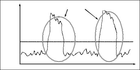
Figure 6-7 illustrates response times in a pattern that shows interference from a special operation.

Figure 6-7 Query performance degrades for a period and returns back to normal

The special tasks can be database internal operations:

Checkpoint

Backup

Smartflow (Advanced Replication) replication operations

HotStandby netcopy or HotStandby catchup

CDC replication operations

Heavy DDL operations

Various aspects exist to optimizing the impact of special operations:

By timing the special operation to occur outside most critical periods.

By optimizing the size of the special task in one way or the other.

In some cases, only simultaneous execution of two or more special tasks cause significantly worse interference than any of the special tasks alone.

The special tasks can also be application batch runs or other tasks that are not present all the time. Logically, application special tasks can be treated similarly to database-related special tasks.

Understand and apply the following aspects when optimizing a special task:

How to control the special task’s execution

How to optimize task execution

How to monitor task execution times

206 IBM solidDB: Delivering Data with Extreme Speed

We examine each special operation in more detail:

Checkpoint

A checkpoint is a task that is executed automatically by the solidDB server process. The checkpoint task takes care of writing all the changed (dirty) blocks in memory back to the disk into the appropriate place in the solidDB database file (or files). The checkpoint task uses CPU to find the dirty blocks inside main memory and relatively heavy disk I/O to write the blocks to disk. Application queries that result in intensive disk I/O are heavily impacted by checkpoints.

By default, a checkpoint is triggered by the write operations counter. Whenever the value of the General.CheckpointInterval parameter is exceeded, the server performs a checkpoint automatically.

To avoid checkpoints entirely, set the General.CheckpointInterval parameter to an extremely large value. Do this only if persistence of data is not a concern.

In heavy write operations, CheckpointInterval can be exceeded before the previous checkpoint completed. To avoid checkpoints being active constantly use the General.MinCheckpointTime parameter.

Another possibility is to execute a checkpoint programmatically with the admin command makecp. This can be advantageous because the application may know about the workload pattern and can pick a more appropriate time to perform a checkpoint operation.

Consider the following aspects:

–How to optimize task execution

By decreasing the General.CheckpointInterval parameter, the size of a checkpoint becomes smaller. The checkpoints, however, become more frequent. It might be that the impact of smaller checkpoints is tolerable; bigger checkpoints disturb the system measurably. In practice, modifications in checkpoint size seldom affect long-term throughput. Theoretically, overall effort in checkpoints is slightly reduced when checkpoints are bigger because of more rows that are possibly hitting the same blocks.

–How to monitor the execution times

The solmsg.out log file contains information about the start and end of each checkpoint. The last entries of solmsg.out can be displayed with the admin command msgs.

The Checkpoint active pmon counter indicates whether a checkpoint is active at that point in time.

The admin command status contains information about write counter values after last checkpoint and gives an indirect indication on whether the following checkpoint is about to occur soon or not.

Backup

In solidDB, backup is a task executed either automatically after setting the Srv.At configuration parameter, or manually/programmatically by the admin command backup. During backup, a full copy of the solidDB database file or files (solid.db) are created in the backup directory. With disk-based tables this essentially means extensive file reading of the source file and extensive file writing at the target file.

Executing the task also requires CPU resources, but predominantly causes congestion in the file system. Running backup has a measurable impact on application performance and response times. It does not block the queries and does not cause disastrously bad performance.

If possible, try to execute backup and application level batch operations consecutively rather than concurrently. This approach is especially true with batch operations that contain long lasting transactions.

Consider the following aspects:

–How to control

Backup process can be started either automatically by timed commands or manually/programmatically by the admin command backup.

–How to optimize task execution

Backup speed depends on the file write speed of the target database. In solidDB, the backup is intended to be stored on different physical devices (to protect against physical failure of the device) than the source database file. Hence, the operation of reading the file and writing the file is not optimized for reading and writing from the same device concurrently.

The most common reason for long lasting backups is the database file size being bigger than it should be, which can be caused by the following ways:

•The database file consisting mostly of free blocks. In solidDB, the disk blocks are not automatically returned to the file system when they are no longer needed. To shrink the database file in size, use the reorganize startup parameter.

•Unnecessary indexes or unnecessary data in the file. In many complicated systems, sizable indexes exist that are never used. Occasionally long backup durations are caused by application level data cleaning tasks having been inactive for long periods of time.

208 IBM solidDB: Delivering Data with Extreme Speed

–How to monitor the execution times

Backup start and completion messages are displayed in the solmsg.out file. There is no direct way of assessing how far the backup task has proceeded. The backup speed can be, however, indirectly calculated by the Backup step pmon counter, based on each backup step passing one disk block of information.

To determine whether a backup is currently active (to avoid starting concurrent batch operations), use the admin command status backup or examine the Backup active pmon counter.

Advanced Replication operations

Advanced Replication, solidDB’s proprietary replication technology, is primarily based on building replication messages inside solidDB's system tables and passing the messages between different solidDB instances. Building and processing the messages can cause database operations related to these system tables.

Finding rows to be returned from the master database to a replica is a similar operation to an indexed select on a potentially large table. If no rows have been changed, a comparable operation is an indexed select returning no rows. For environments with multiple replicas, the effort must be multiplied by the number of replicas.

When moving data from replica databases to the master, the additional load in the replica consists of the following actions:

–Double writing (in addition to actual writes, the data needs to be written in a propagation queue)

–Reading the propagation queue and writing to system tables for message processing

–Processing the message in system tables and sending to the master

The master database processes the message in its own system tables (inserts, selects and deletes) and re-executes the statements in the master (essentially the same operations as in the replica).

To fully understand Advanced Replication's impact on system performance, you should understand its internal architecture. See the Advanced Replication User Guide at the following location for more information:

http://publib.boulder.ibm.com/infocenter/soliddb/v6r5/nav/9_1

Consider the following aspects:

–How to control

All replication operations (that is, replica databases subscribing to data from master databases and replica databases propagating data to master databases) are controlled by commanding replication to take place with SQL extensions at the replica database. The application has full control of initiation of replication. Heaviness of each operation is naturally caused by the amount of changes in the data between replication operations. Advanced Replication enables defining the data to be replicated by publications. Publication is defined as a collection of one or several SQL Result Sets.

–How to optimize task execution

The impact of replication depends on the number of rows to be replicated by a single effort. It is possible to make the impact of refreshing an individual publication smaller by breaking publications into smaller pieces as follows:

•Creating several publications and defining different tables in different publications

•Refreshing only part of a row (by key value) by individual subscribe effort

These changes make the performance hits smaller but more frequent. The numbers of rows that are replicated are not affected. Timeliness of replicated data can suffer.

For systems with a high number of replicas (with high number of tables to be replicated), the polling nature of Advanced Replication start to cause load at the master database. For each replica and each table to be replicated, an operation equivalent to selection can be executed in the master database even if there are no changes in data. Overhead that is caused by this phenomenon can be reduced by adjusting the replication frequency, which results in an adverse affect on the timeliness of the data.

–How to monitor the execution times

The SQL commands that trigger the replication can be traced in the replica database’s soltrace.out file like all the other SQL commands. The level of

replication activity in both replica and master databases can be measured by a set of pmon counters. Pmon counters starting with the word Sync are related to Advanced Replication.

HotStandby netcopy or HotStandby catchup operations

In HotStandby, primary and secondary databases must run in Active state where every transaction is synchronously executed at the secondary

210 IBM solidDB: Delivering Data with Extreme Speed

database also. Before reaching active state, the secondary database must perform the following tasks:

–Receive the database file from the primary database

–Receive the transactions that have been executed since the databases were connected and process them

While the secondary database is in the process of receiving netcopy or processing catchup, it is not able to process requests at all. Also, sending the entire file or just the last transactions will cause load at the primary database and interfere with perceived performance of the primary database also.

HSB Netcopy is an operation quite analogous to a backup. It might lead to heavy disk read I/O at the primary database and interfere heavily with other intensive database file read I/Os.

HSB Catchup is essentially about rerunning the transaction log. If the transactions that were written during the time that the primary and secondary were disconnected exceed the buffer size, log file reads must be executed at the primary database. In reality, this interference seldom causes measurable problems.

Consider the following aspects:

–How to control

Both HSB netcopy and catchup are operations that are executed by SQL at the primary database. This might be visible to the application or hidden by the Watchdog application or HAC module.

–How to optimize task execution

The level of interference caused by these operations can be tuned by the HotStandby.CatchupSpeedRate configuration parameter.

–How to monitor the execution times?

Both catchup and netcopy start and completion messages are logged in the solmsg.out file.

The database states of primary active and secondary active indicate that neither netcopy nor catchup are in progress. The states are visible in the HSB state pmon counter.

CDC Replication operations

CDC is a replication technology included as part of the solidDB Universal Cache product to facilitate data transfer and synchronization between solidDB and the back-end database.

The CDC replication process can cause some load on the databases and that can potentially interfere with perceived application performance.

Essentially, CDC is based on two parts, capture and apply:

–Capture reads log entries from a virtual log table (in solidDB's case, SYS_LOG)

–Apply converts the log entries to SQL statements which get executed in the target database.

The reading from the virtual table SYS_LOG is implemented as reading from an in-memory buffer and, thus, can inflict a significant load. When the connection is broken and log operations occur, a catch-up situation results upon the next enablement of the solidDB InfoSphere CDC replication engine. In that situation, some I/O overhead may be observed until catchup completes.

CDC replication can lead to disastrous impact on performance when throttling is activated. This means that the target database has been too slow to accept applying the captured changes. To avoid the virtual log size growing too big, the server will slow down new write operations. The read-only load is unaffected by the throttling. Because the log reader operates in an asynchronous mode with respect to transactions (that is, it reads only committed transactions), no locking-related performance degradation is possible.

Consider the following aspects:

–How to control

CDC configuration is performed with dedicated CDC tools. After the replication process is set, it can be controlled (started or stopped) both with GUI tools or with shell level commands, such as dmts64 or dmshutdown. There are no solidDB controls to stop the replication. If there is a need to stop the replication, use the CDC instance configuration tool or the shutdown shell command. Any other way to stop the replication (such as stopping users) may damage the replication setup.

The throttling is enacted when an in-memory buffer is filled up. The size of the buffer can be controlled with the configuration parameter LogReader.MaxSpace (in number of log records). The factory value is 100000.

–How to optimize

Relatively few things must be done to optimize replication in the capturing database. In the database that receives the transactions being applied by CDC, you can use regular write optimization options such as:

•Removal of unnecessary indexes. CDC does not force index structures in source and target databases to be identical.

•Optimization in transaction logging mode.

212 IBM solidDB: Delivering Data with Extreme Speed

–How to monitor

The status of throttling may be monitored with the Logreader spm freespc pmon counter. When it reaches zero, the throttling is enabled.

Other CDC-based activity can be monitored by several other pmon counters. All of them are labeled Logreader.

Write operations executed by CDC when applying the captured data are visible through regular pmon counters (such as SQL Execute and DBE Insert).

Heavy DDL operations

Data Definition Language (DDL) operations, such as ALTER TABLE and CREATE INDEX can cause interference as follows:

–Potential heavy disk activity that interferes with concurrent operations that are related to other tables, which are not directly involved in the DDL operation

–Blocking the related table (or tables) for the duration of the operation Consider the following aspects:

–How to control

Running DDL is entirely triggered by executing SQL components external to the database.

–How to optimize task execution

DDL operations are potentially heavy. Only limited means are available for optimization:

•DDL-operations are executed as write operations, which includes a write to the transaction log file also. Disallowing new connections with the admin command close command, turning logging off (possibly along with other changes in configuration as suggested below), running the DDL, re-enabling logging, and opening the server back up to new connections with the admin command open can be faster than just running the DDL.

•With disk-based tables, having a bigger cache (setting IndexFile.CacheSize) size can speed up most DDL operations.

•With both main memory tables and disk-based tables, the disk block size (the IndexFile.BlockSize configuration parameter) affects checkpoint duration.

Note: The optimal block size for minimizing the duration of index creation is not necessarily the optimal size for speed of index usage or regular application usage