4. Principle of rational approximation

In the principle of rotational approximation, a desired frequency is measured by comparing it with a standard frequency. However, not by simple pulses count in a time sample, but using the special mathematic framework introduced in [16-18]. The zero crossings of both frequencies are detected, forming two regular independent narrow pulse trains (see Fig. 7). The desired and standard trains of narrow pulses are compared for coincidence. This comparison is made using an AND gate. A coincidence pulse train is generated. The coincident pulses can be used as triggers to start and stop a pair of digital counters(see Fig. 8).

The standard and desired pulse trains are applied to the counters and a measure of the desired frequency is obtained by multiplying the known standard frequency by the ratio of the desired count and the standard count obtained with the two digital counters P and Q. Consider as the desired or unknown frequency andas the standard frequency.

Fig.7. Process of direct frequency comparison: geometric theory of coincidence transformation.

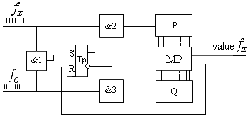
Fig.8. The frequency meter block diagram.

In Fig. 7, andare the unknown and standard trains of narrow pulses, respectively,with frequencies f_x and f₀. The pulses widths in both trains of Fig. 7 are τ. Consider as the greatest common divisor (gcd) of both periodsand.represents a minimally distinguishable time interval and indirectly a quantum, which as shown below, is defined by the stability of the standard frequency.andare independent parameters (this must to be a keynote for any simulation of this process).

There exists a pair of narrow pulses in the pulse trains which exactly coincide on the time axis. This first, completely coincident pair of pulses (Fig. 7) is designated with zero indexes. This pair pulses is a command to start the frequency measurement by device presented on Fig.8.

Correspondingly to the mentioned above, both unknown and standard frequencies f_x and f₀ are input to the circuit. &-gate &1 verifies the coincidences in time domain between trains and, and opens count of pulses by independent counters P and Q (on Fig.8) at the first coincidence using RS-trigger. Microprocessor MP controls this process by set/reset of RS-trigger when each next coincidence occurs (see real-time process on Fig.7).

andare the numbers of counted pulses from theandsequences that occur between adjacent coincidences.MP (Fig.8) saves in memory independently all values of pairand on each n-th coincidence occurrence. Between two completely coincident pairs (see Fig.7), which correspond to pulses number 0 and 17 of the reference frequency sequence , there also exist some partial coincidences. Adjacent coincidences may be either partial or total. The indexn refers to either partial or total coincidences.

For the considered particular example in Fig. 7, for the second and the third partially coincident pairs, respectively:

(1)

Fractions ,each independently can be used for an estimation of the unknown frequency. In this case, both of these values are better approximation to measured parameter of any automotive FDS sensors (see Fig. 3), than the value obtained in a classical measurement algorithm (Fig.1).

On the other hand, if we have any two fractions, they can form a mediant fraction as follows [16, 38]:

(2)

Thus, in our case andare approximants to each other and to the mediant formed by them. That is,

(3)

The mediant and its approximants have the following common fundamental property:

(4)

The mediant can be generalized in this form

(5)

where n is the number of the fraction and m is the number of the mediant, both written in parenthesis in (5). According to the definition in [36, 37], the mediant is the fraction formed by two fractions andin the next way:

[mediant fraction] =

Thus, a mediant can be formed with a minimum of two fractions. In this case, the number of the fractions is n=2 and the corresponding number of the mediant is m=1. That is, the number of the mediant is always one unit less than number of the fraction under consideration.

The mediant also can be formed by three fractions with numbers n=1, 2, 3 ([mediant fraction] = ). In this case their mediant is formed by the last fraction (n=3) and the previous mediant of the fractions n=1 and n=2.

From (5) we can consider two sums:

- sum of numerators of all n fractions, which form the mediant m.

- sum of denominators of all n fractions, which form the mediant m.

These sums automatically provide back-to-back continuous (without dead-time) averaging throughout the measuring time. The ratio of the frequencies can be considered as an irrational number,. Since the mediantis closer to α, than its forming fractions, it is possible to accept, and

, (6)

where f_xm is the approximation of unknown frequency value f_x by the m-th mediant.

The relative value of the systematic measurement error(frequency offset) using (6) can be written as follows:

(7)

In [19, 20], it has been shown that approximants and their mediants can be used to directly compare an unknown frequency with a known one. Using approximants and their mediants the value of unknown frequency and its systematic error can be defined.

In a sequence of mediants

(8)

it is possible to choose one [16, 19] that satisfies (5) in this way (9)

By means of the gcd , it is possible to represent the periodsby numbers. Then,is a common multiple.

Thus, we have , the accepted decimal notation that the mediant, which provides the best approximation forand the greatest possible accuracy for, has a numerator of the form.

This feedback signal resets the trigger to initial state. It means the numerator is in the form of “one with r zeros” and it is easy to achieve a desired accuracy in hardware counting of least significant bits in counter P. This is a stop signal for the end of the measurement process and it allows constructing time keeping systems or frequency meters with set accuracy and duration of measurements.

At the same time, the measurement of the parameter of any automotive FDS (see Fig. 3), converted into proportional frequency (or nominal frequency changes Δf), is finished too. In [16], it is proved that at this moment the readout result in the counter is the best proportional approximation of measured frequency true value on the given interval of time.

At this point, it is expedient note that the absolute time of such measurement is significantly less than the result of the classical method mentioned in Fig.1 and in [3]. In fact, for any classical frequency count method the time sampling interval is 1s as a rule and it has associated a “±1 count error” (i.e., the quantization error of ±1 cycle) [3, 16]. Whereas the method of rational approximation presented in this paper has shorter time of measurement.