Table 6.1. Using the Keyboard to Navigate Excel

Press This Key…	To Move To
Arrow keys	The direction of the arrow one cell at a time
Ctrl+up arrow, Ctrl+down arrow	The topmost or bottommost cell that contains data or, if at the end of the range already, the next cell that contains data
Ctrl+left arrow, Ctrl+right arrow	The leftmost or rightmost cell that contains data or, if at the end of the range already, the next cell that contains data
PageUp, PageDown	The previous or next screen of the worksheet
Ctrl+Home	The upper-left corner of the worksheet cell A1
End, arrow	The last blank cell in the arrow's direction
Ctrl+PageUp, Ctrl+PageDown	The next or previous worksheet within the current workbook

To Do: Create Your First Worksheet

The next hour's lesson presents the details of creating, editing, and understanding specific areas of an Excel worksheet. For practice, however, work through the following steps to try Excel now. To do so, you will create a simple test-tracking worksheet for a professor. By working with a hands-on example now, you'll have a better feel for the overall Excel concept as you work the rest of this section of the book.

Follow these steps to create your first worksheet:

1. Select File, New and select Blank Workbook from the New Worksheet task pane to create a new workbook.

2. Click on cell C4 to move the cell pointer there and make it the active cell. The cell name, C4, appears in the formula bar.

3. Type Student Gradebook . The text is wider than the cell, but Excel extends the text label over into the right cell (D4).

4. Click on cell B6 and type Name .

5. Press Tab to move the cell pointer to C6. (You can also click in C6 or press the right-arrow key to move the cell pointer to C6.)

6. Enter the labels Test 1, Test 2, Test 3 , and Average in cells C6 through F6.

7. Move to B8 and enter these values across row 8: Mary Bee, 77, 89 , and 86 . (The 86 ends up in cell E8.)

8. Enter these values underneath the previous ones to add the second row of data for your worksheet: Paul North, 89, 87 , and 94.

9. Enter the following data for the next row: Terry Smith, 93, 100 , and 95 . Notice that cell B10 is not wide enough to hold Terry Smith's entire name. As soon as you enter data in C10, the right portion of Terry Smith's name is truncated. You will fix this problem in a moment.

10. Enter the following for the row 11: Sue Willis, 64, 79 , and 83 .

11. Type Class Average: in cell D13. (The label will flow into E13.) Your worksheet should resemble the one in Figure 6.6.

Figure 6.6 You are on your way to creating your first Excel worksheet!

To Do: Format the Worksheet

The worksheet requires some formatting to look better, but you've already used Excel to enter text and numbers. The averages now need computing via a formula. Additionally, a little formatting would greatly improve the look. Follow these steps to complete the worksheet:

1. Move the cell pointer to F8 and type this: =(C8+D8+E8)/3 . Then, press the down arrow to move to cell F9. Notice that Excel computed the average of Mary Bee's test scores. You just entered a formula that requests the average. The formula tells Excel to add the contents of cells C8, D8, and E8 and then divide the sum by 3. Several methods exist for creating such a formula, and you'll learn even better ways throughout the next three hours' lessons.

2. Excel is smart and guesses at a lot of tasks to make life easier for you. Instead of typing the same formula all the way down column F, you only need to copy and paste the formula you just entered to F9, F10, and F11 to calculate the other three student averages. Click on cell F8 (the cell to copy), and press Ctrl+C to copy the cell to the Clipboard. Excel highlights the cell to show the selection.

3. Click cell F9 and do this: Hold down the Shift key while pressing the down arrow twice. Excel highlights three cells. These cells are the target of your copy.

4. Press Ctrl+V (or select Edit, Paste) to paste the Clipboard contents into the highlighted cells. When you do, Excel instantly updates the averages for the remaining three students. Excel even changes the formula you copy to reflect the new row numbers. This is called relative cell referencing because the formulas are copied relative to their new locations. You can ignore the Paste icon that Excel displays after the paste. When you paste data into a document, the Paste icon appears and enables you to modify the way the paste is performed. You can, for example, elect to paste the formula as text, and if you do, the result does not show in the cell but the formula itself does.

Note

If Excel refused to change the row numbers when you copied the formula from F8, all four students would reflect Mary Bee's average. You can click on cell F10 and look at the formula in the formula bar (beneath the standard toolbar) to see that all references now indicate row 10 and no longer row 8 even though you copied the formula from row 8. Fancy? You bet.

5. You now must compute the average for the class. That's simple: just type the following formula in cell F13: =(F8+F9+F10+F11)/4 . The class average appears instantly. Your worksheet now looks like the one in Figure 6.7.

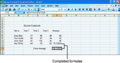
Figure 6.7 Excel calculates all the averages for you.

Now that you've finished entering text, numbers, and formulas, you can improve a worksheet's look with a little formatting. In addition, you might be interested in knowing how Excel can improve the functionality of the worksheet. If you insert new blank rows into the worksheet, Excel changes the average calculations at the end of the displaced student rows to reflect their new row location. You also can insert new columns in case the students take additional tests, and the formulas update to reflect new column names.