Computer Science АС (ГСФ) / CS Work at lab classes / 5 Intro Excel - Formatting

Microsoft Excel - Lists

1. In cell A1, type the title for your spreadsheet: Top 20

2. In cell A2, type: VH1

3. In cell A3, type these dates: 12/14/08-12/21/08

4. Starting in cell A5, enter this data into your spreadsheet:

Position	Artist	Title
1	David Archuleta	Crush
2	David Cook	Light On
3	Britney Spears	Womanizer
4	AlterBridge	Watch Over You
5	Beyonce	Single Ladies
6	Kid Rock	Roll On
7	Jennifer Hudson	Spotlight
8	Safetysuit	Someone Like You
9	Lifehouse	Broken
10	Katy Perry	Hot n Cold
11	The All-American Rejects	Gives You Hell
12	Beyonce	If I Were a Boy
13	Coldplay	Lovers In Japan
14	Eric Hutchinson	Rock & Roll
15	Rihanna	Rehab
16	O.A.R.	Shattered
17	The Killers	Human
18	Missy Higgins	Where I Stood
19	Fall Out Boy	I Don’t Care
20	Pink	Sober

5. Format the list in any way that you want.

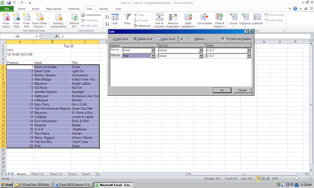
6. Highlight your chart from A5 to C25. From the Datatab, select Sort. The 'Sort' window will appear.

7. Make sure that the box that says “My Data has Headers” is selected at the top right of the Sort window

8. Click on the down arrow in the 'Sort By' box. A list of your column titles will appear. Choose Artist.

9. Click on “Add Level”, when the Then By box appears, click on the down arrow and choose Title.

10. Click OK.

11. The list should be sorted alphabetically by artist and then by song title.

12. Click the Undo button (Found in top left corner)

We can filter lists so that only certain information is displayed.

1. Click on any cell in your chart below Row 5.

2. In the Data tab, click Filter.

3. Arrows should appear next to each column heading.

4. Click the down arrow to the right of the Artist heading.

5. Select onlyBeyonce, by unchecking the box next to “select all” and checking the box next to Beyonce

6. You should only see two songs in your list ("Single Ladies" and "If I Were a Boy").

7. Click on the down arrow to the right of Artist again.

8. Choose (Select All).

9. Your list should look complete again.

Imagine we want to filter the list to see the Top 10 songs for the week.

10. Click the down arrow next to Position, select Number Filters and Top 10.

1

2

3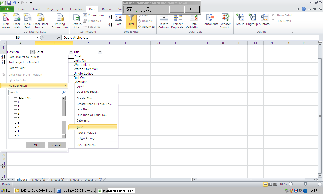

11. Choose (Top 10…). You should see a dialog box come up.

12. Click OK.

13. The songs 11 through 20 will be displayed because these are the highest numbers. This isn’t the Top 10 we want!

14. Click on the down arrow by Position, and then click on the box next to Select All

15. Click OK. Your list should look complete again.

16. Again click on the down arrow next to Position.

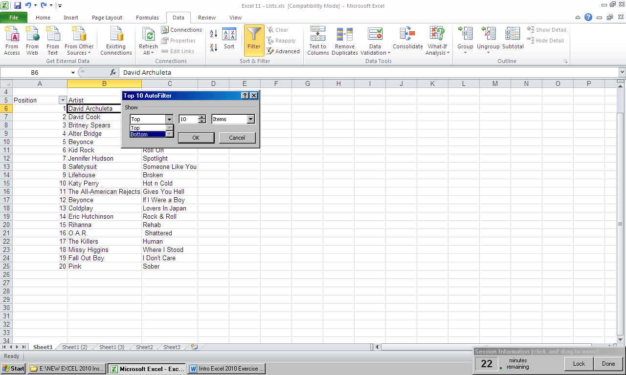
17. Click on Numbers Filter and then select Top 10

18. This time, in the dialog box, use the down arrow and change Top to Bottom.

19. Click OK.

20. The list should show songs 1 through 10 now.

21. Save your work as Exercise 7.

Exercise-Advanced Functions

Imagine you have been asked to create a spreadsheet for Mr. Blogg, a teacher, so he can keep track of his students and their grades.

1. Type “Joe Blogg’s High School Class” in cell A1.

2. Type “2009 Student Grades” in cell A2.

3. Enter this raw data as follows:

Student	Term 1	Term 2	Term 3	Term 4
Jean Peterson	15	12	14	17
John Archer	18	14	17	16
James Smith	23	22	19	21
Chris Pearson	8	11	7	6
Jeff Sinclair	19	19	18	14
Kathryn Jackson	13	12	10	12
Ben Coleman	16	22	20	19
John Sheridan	22	20	24	21
Lisa Alexander	23	21	28	21

4. Format the chart however you wish. If you want to, you can use the Autoformat option.

5. In cell A14, type AVERAGE.

6. In cell F3, type YEAR TOTAL.

7. Complete the addition for each student’s yearly total.

8. Click in cell B14.

9. Type =AVERAGE(B4:B12). Make sure all the Term 1 grades are highlighted.

10. Press Enter. You should get the answer. 17.44444.

11. Calculate the average for Terms 2, 3, 4 and the Year Totals as well.

Using an If Function

An If function selects from two different possibilities based on criteria that you supply. In this grades example, we will create an If function that determines if each student is passing or failing. A student will pass if their total grade is at or over 50, and will fail if their grade is below 50.

1. Click in cell G3 and type Pass/Fail.

2. Click in cell G4.

3. Enter the following: =If(

4. Type: F4>=50

   1. This asks if F4 is greater than or equal to 50.

5. Type a comma.

   1. Commas separate functions into sections.

6. Type“Pass” in quotation marks.

   1. This specifies that if the first section is true (F4 is greater than or equal to 50), the textPass will be displayed.

7. Type a comma.

8. Type “Fail” in quotation marks.

   1. This specifies that if the first section is false (F4 is less than 50), the text Fail will be displayed.

9. Type a closing parenthesis.

10. The equation should look like this:=If(F4>=50,”Pass”,”Fail”)

11. Press Enter.

12. You can use the fill handle to calculate all of the If functions.

13. If you see a mistake, look in the formula bar and make any corrections.

Using a LookUp Function

Lookup functions allow Excel to choose from several different options in a table. We will use a lookup function to determine each student’s letter grade.

1. Complete this table in cells G17 to H21.

0	F
35	D
50	C
65	B
80	A

2. Click in cell H3 and type Grade.

3. Click in cell H4.

4. Enter the following =VLOOKUP(

   1. The V stands for Vertical. You can also do a horizontal lookup depending on the type of table you create.

5. Type F4 (the cell with Jean Peterson’s yearly total)

6. Type a comma to end the first section.

7. Highlight cells G17 to H21 (the grades table)

8. Press the F4 function key at the top of your keyboard. K4:L8 will change to look like $K$4:$L$8.

   1. This is called absolute referencing. Excel usually uses relative referencing. When you used the fill handle to complete all of the If functions earlier, the cells the formula referred to changed to fit each new location.

   2. For this formula, we always want to refer to cells K4:L8, even when we calculate grades for a different student.

   3. The first section where you typed F4 is not absolute, it is still relative. That is because we DO want the first section (the yearly total) to change as we calculate grades for DIFFERENT students.

9. Type another comma and then the number 2.

   1. The number 2 refers to the fact that the grades table (K4:L8) is a two-column table and the answers we want are in the second column (the letter grades).

10. Type another comma and then the word TRUE.

1. Typing the word TRUE tells Excel that if an exact match for a number can’t be found in your grades table, to find the closest match instead.

1. The complete formula should look like:

   1. =VLOOKUP(F4,$K$4:$L$8,2,TRUE)

2. Press Enter.

3. Use the fill handle to find the letter grades of each student.

4. Your students should have 3 A’s, 3 B’s, 1 C, 1 D and 1 F.

5. If it doesn’t seem right, check your equation in the formula bar and make corrections if necessary.

8