

§ 3.9. Other Remarkable Limits
Consider the following limits of functions often encountered in applications:
(1)
![]() ,
(7)
,
(7)
(2)
![]() for
a=e,
for
a=e,
![]() .
(8)
.
(8)
(3)
![]() .
(9)
.
(9)
Proof.
1.
![]() .
.
2. Define ax–1=t as x0, t0, ax=t+1 . Take the logarithm of both terms by definition of a: x=loga(1+t), substitute in (8), and, according to (7), obtain:
![]() .
.
3.
Define the numerator
(1+x)–1=t,
(1+x)=1+t
as
x0
t0.
Take
the logarithm of both terms by definition of e:
![]() ,
multiply
the numerator and the denominator of limit (9) by the obtained
expression
,
multiply
the numerator and the denominator of limit (9) by the obtained
expression
![]()
![]() .
.
Remark. Here the author uses the words of his ex-student: “The limit is like water which penetrates everywhere”, i.e., the limit penetrates into a sum, a product, a quotient of limits, an argument of functions, in powers, under the radical sign and logarithm, etc..
§ 3.10. Continuity of Functions
Define f(x) in a neighborhood of х0 .
Definition 1. If the left and the right limits coincide and equal the value of a function at point х0, then the function f(x) is said to be discontinuous at point х0
![]() .
(10)
.
(10)
y
f (x0)
0 x0 x
We attach the increment х to an argument x. Then the function must also obtain the increment у:
|
у=f(x0+x)–f(x0).
|
f(x0+x)
f(x0)
0 x0 x0+x x |
 у
у
Definition 2. If the small increment of an argument corresponds to the small increment of x, then this function is said to be continuous at this point
![]() .
(11)
.
(11)
![]() .
.
These two definitions are equivalent, i.e., it is possible to obtain the second definition from the first and vice versa. (Prove this on your own).
Definition. The function is said to be continuous on a domain if it is continuous at each point of this domain.
All
elementary functions are continuous. Elementary functions are denoted
by
![]() .
.
Example 1. Prove that f(x)=cosx is a continuous function on the whole x-axis.
Use the second definition of the function continuity (11). We find the limit of function increment
y=f(x+x)–f(x), f(x+x)=cos(x+x),
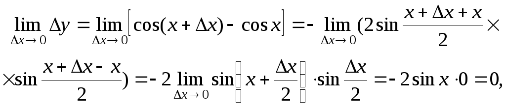
i.e., the condition of the second definition of continuity is satisfied.
Example
2.
Prove
that y=tanx
is continuous on the interval
![]() .
Use
the second definition of continuity:
.
Use
the second definition of continuity:
![]() ,
,
![]() =
=![]() =
=
=![]() =
=![]() =
=![]() =0.
=0.
Consequently, the function is continuous.
3.10.1.
The classification of the points discontinuities. The
discontinuities can
appear only if the conditions of continuity, the condition (10) are
broken, i.e.,
![]() ,
х0
is
the point, where (10) is not satisfied.
,
х0
is
the point, where (10) is not satisfied.
Definition.
A simple discontinuity is such a point, at which there are one-sided
limits and
![]() ,
but they are not equal:
,
but they are not equal:
![]() .
.
|
y B
A
0 x0 x |
|
E
 xample
3.
у
xample
3.
у
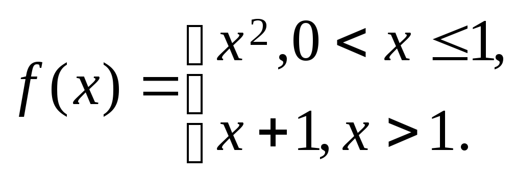

 y=x2
y=x+1
y=x2
y=x+1
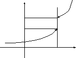
is a simple
discontinuity

0 1 х
Find the left limit of a point х=1:
![]() .
.
Find the right limit:
![]() .
.
The limits do not coincide; thus, we have the simple discontinuity at the point х=1.
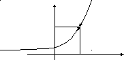
Definition. A point х=х0 is called a removable continuity if the left and right limits exist and equal, but the function is not determined at this point.
f(x0–0)=f(x0+0), f(x0)-?
Remark.
Such a point can be removable if we take the value of limit
![]() for f(x0).
for f(x0).
Example 4. Find the discontinuity of
![]() .
The
value of the function does not exist, because
the
denominator equals zero as
х=5,
but the limit exists:
.
The
value of the function does not exist, because
the
denominator equals zero as
х=5,
but the limit exists:
![]()
![]() 10,
10,
The point х0=5 is a removable discontinuity; we supplement the function with f(5)=10.
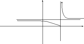
Definition. The discontinuity of the second kind is a point, where at least one of the one-sided limits either does not exist or equals the infinity.
 у
у
0 х0 х
![]()
Example 5. Test the following function for the discontinuity:
![]()
 .
у
.
у
Find the left limit
![]() .
.
0 х
Respectively, the right limit is
![]() .
.
Both limits do not exist; the function has the discontinuity of the second kind at the point х=2.
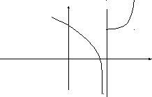
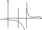
Example
6.
Consider
![]() for
the discontinuity at the points
х1=3,
х2=0.
for
the discontinuity at the points
х1=3,
х2=0.
We
find the value of a function at the point х0=0
;
![]() =
=![]() ;
thus,
the function is continuous at the point
х=0.
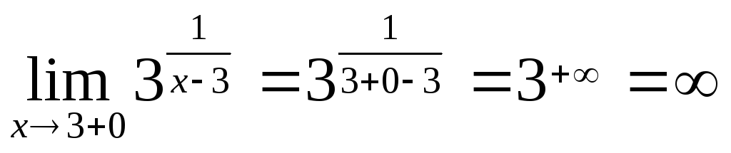
At
the point
х0=3,
;
thus,
the function is continuous at the point
х=0.
At
the point
х0=3,
![]() ,
we
find
,
we
find
![]() ,
,
 .
.
 у
у
1
х=3 is a discontinuity
of the second kind. 0 3 х
3.10.2. Theorems on continuous functions. The first Cauchy-Bolzano theorem. If f(x) is defined and continuous on the interval [a;b] with different signs at the ends of this interval, then there is at least one point х=с, where f(c)=0. (Without proof).
T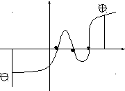 his
theoremcan
be represented graphically as is:
his
theoremcan
be represented graphically as is:
у
а
0 с1 с2 с3 b х
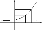
The second Cauchy-Bolzano theorem. If f(x) is defined and continuous on the interval [a;b] with different values at the ends, then any value of a number М has the point х= с between these values; thus, f(c)=M is satisfied. (Without proof).
f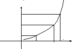 (a)=A;
f(b)=B, AB.
(a)=A;
f(b)=B, AB.
у
A<M<B. B
M
A
0 a c b х
The Weierstrass theorem. If a function is defined and continuous on the interval [a;b], then it is limited from above and below on this interval, i.e., mf(x)M.
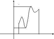 y
y
M
m
0 a b x
3.10.3. The comparison of infinitesimals. Suppose that there are the following infinitesimals (х) and (х), i.e.,
![]() ,
,
![]() .
.
Definition. If there is the ratio limit between these infinitesimals equal to zero
![]()
then the infinitesimal (х) is said to be of a higher order than (х).
Notation: =0().
Definition. Two infinitesimals (х) and (х) are infinitesimals of the same order if their ratio limit equals a constant number
![]()
Definition. If the ratio limit of infinitesimals equals 1 then the infinitesimals (x) and (x) are said to be equivalent.
Notation: (х) (х).
Definition.
If
limit
![]() does not exist,
then these two infinitesimals are said to be nonmesuarable.
does not exist,
then these two infinitesimals are said to be nonmesuarable.
Theorem.
To
equal two infinitesimals
(x)
and
(x),
it is necessary and sufficient that
![]()
exists.
Examples.
(1).
![]() ,
,![]() .
The
sine of a small-angle is equivalent to the
.
The
sine of a small-angle is equivalent to the
angle itself.
(2).
![]() ,
,
![]() .
.
(3).![]()
 ,
,![]() .
.
(4). ![]()
![]()
![]()
![]() .
.