

§ 3.5. Fundamental Theorems on Limits
Theorem I. The limit of the algebraic sum of finitely many functions equals the sum of the limits of these functions:
![]() .
.
Proof.
For
simplicity, we shall prove the theorem for the sum of two functions.
Suppose that
![]() .
By Theorem I, these functions can be represented in the form
u1(x)=b1+1(x),
u2(x)=b2+2(x),
where
1(х),
2(х)
are
infinitesimals. Consider the sum
.
By Theorem I, these functions can be represented in the form
u1(x)=b1+1(x),
u2(x)=b2+2(x),
where
1(х),
2(х)
are
infinitesimals. Consider the sum
u1(x)+u2(x)=b1 +b2+1(x)+2(x), where 1(x)+2(x) is infinitesimal.
Using the second part of Theorem I, we obtain
![]() ,
as required.
,
as required.
Theorem II. The limit of the product of two functions equals the product of the limits of these functions:
![]() .
.
Proof.
Suppose
that
![]() and
and ![]() .
By Theorem I, we have u1(x)=b1+1(x)
and
u2(x)=b2+2(x).
.
By Theorem I, we have u1(x)=b1+1(x)
and
u2(x)=b2+2(x).
Consider the product
u1(x).u2(x)=b1.b2+b12(x)+b21(x)+ 1(x)2(x)=b1.b2+(x),
where
(х)
is
the infinitesimal sum of the last three terms. Theorem I implies
![]() ,
as required.
,
as required.
Theorem III. The limit of the ratio of two functions equals the quotient of the limits of the numerator and the denominator:
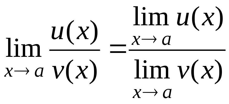 .
.
Proof. Suppose that
![]() .
.
Then
u(x)=b1+1(x) and v(x)=b2+2(x).
Consider the quotient and transform it by reducing to a common denominator:
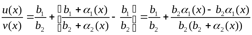 .
.
It is easy to show that the second quotient is infinitesimal. The fundamental Theorem I implies the required assertion.
Theorem IV (the sandwich theorem). If, in a neighborhood of a point а, the inequalities
u (x) z (x) v (x) (3)
hold
![]() ,
then limit
of z(x)
exists and equals
,
then limit
of z(x)
exists and equals
![]() .
.
Proof.
Subtracting b
from
inequalities (3), we obtain (x)–b
z(x)–bv(x)–b.
By definitions, if |x–a|<,
then
|u(x)–b|<
and
|v(x)–b|<;
hence –<u(x)–b<,
and
–<v(x)–b<
. Therefore, for all
|x–a|<,
we
have
–<z(x)–b<,
or
|z(x)–b|<,
which
means that
![]() .
.
Theorem
V. If
a function f(x)
is
monotonically increases (decreases) and is bounded as
х
а
above
(below), then f(x)
has
a finite limit
![]() (Without proof.)
(Without proof.)
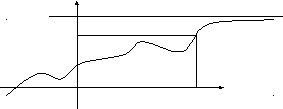 y
y
M
y=f(x)
b
0 a x
3.5.1. Computations of limits. Examples.
I. Limits as x.
(1)
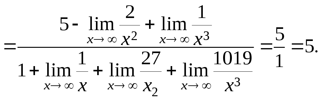
The limits in the numerator and the denominator equal zero.
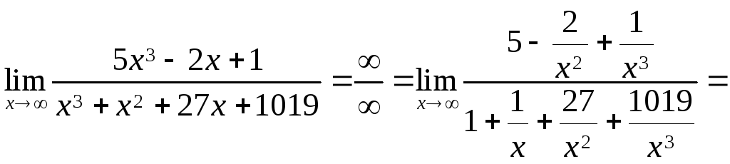
To find the limit of a linear-fractional function, we must divide the numerator and the denominator by х to the maximum power among the powers of x in the numerator and the denominator.
(2)
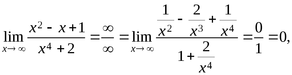
because х4 is the maximum power of x in the numerator and the denominator.
(3)
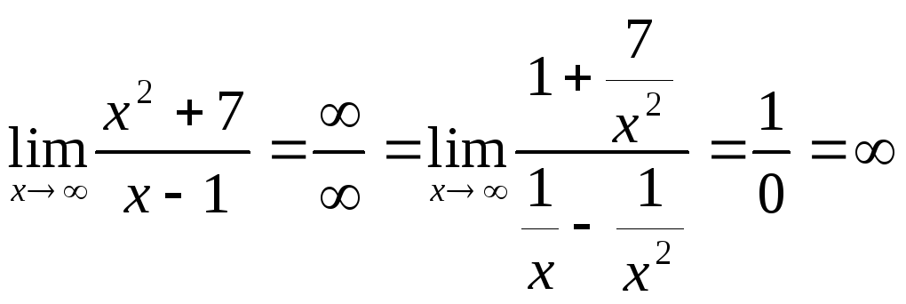 (divide
by
х2).
(divide
by
х2).
A simple method for finding limits of linear-fractional functions as х is to leave the term containing the maximum power of х in the numerator and the denominator:
4)
![]() ,
,
5)
![]() ,
,
6)
![]() .
.
Let us find limits (1), (2), (3) by the simple method:
![]() ,
,
![]() ,
,
![]() .
.
Deleting the terms containing lower powers of x from the numerator and the denominator is only possible because, after division by х to the maximum power, the limits of all such terms vanish.
II.
Limits
as
ха.
Looking
for a limit, first, substitute
![]() in the function. If we obtain a number, then this number is the limit
of the function. If we obtain one of the indeterminacies
in the function. If we obtain a number, then this number is the limit
of the function. If we obtain one of the indeterminacies
![]() ,1,
and
,1,
and
![]() ,
then we must eliminate it by transforming the function and then to
pass to the limit.
,
then we must eliminate it by transforming the function and then to
pass to the limit.
(1)
![]() ,
,
(2)
![]() ,
,
(3)
![]() ,
,
(4)
![]()
![]() .
.