EViews provides various degrees of support for the analysis of data in panel structured workfiles.
There is a small number of panel-specific analyses that are provided for data in panel structured workfiles. You may use EViews special tools for graphing dated panel data, perform unit root or cointegration tests, or estimate various panel equation specifications.
Alternately, you may apply EViews standard tools for by-group analysis to the stacked data. These tools do not use the panel structure of the workfile, per se, but used appropriately, the by-group tools will allow you to perform various forms of panel analysis.
In most other cases, EViews will simply treat panel data as a set of stacked observations. The resulting stacked analysis correctly handles leads and lags in the panel structure, but does not otherwise use the cross-section and cell or period identifiers in the analysis.
Panel-Specific Analysis
Time Series Graphs
EViews provides tools for displaying time series graphs with panel data. You may use these tools to display a graph of the stacked data, individual or combined graphs for each crosssection, or a time series graph of summary statistics for each period.
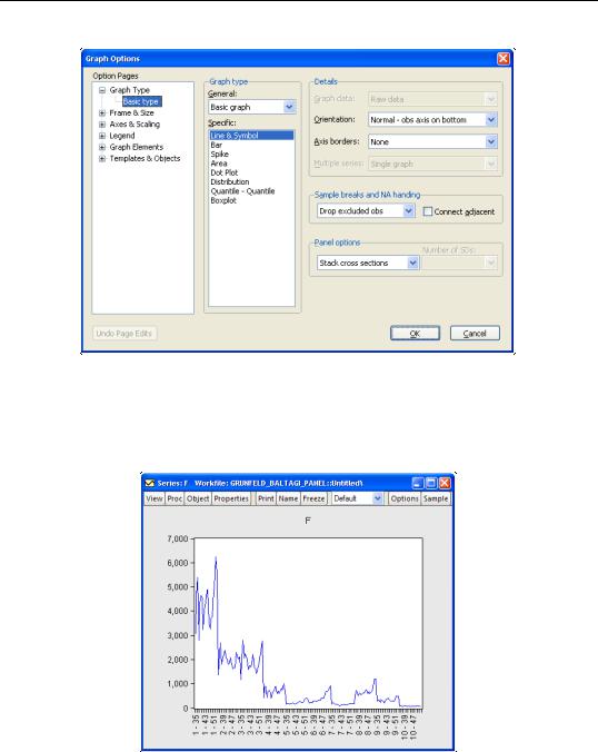
To display panel graphs for a series or group of series in a dated workfile, open the series or group window and click on View/Graph... to bring up the Graph Options dialog. In the Panel options section on the lower right of the dialog, EViews offers you a variety of choices for how you wish to display the data.
636—Chapter 36. Working with Panel Data
Here we see the dialog for graphing a single series. Note in particular the panel workfile specific Panel options section which controls how the multiple cross-sections in your panel should be handled. If you select Stack cross sections EViews will display a single graph of the stacked data, labeled with both the cross-section and date. For example, with a Line & Symbol type graph, we have
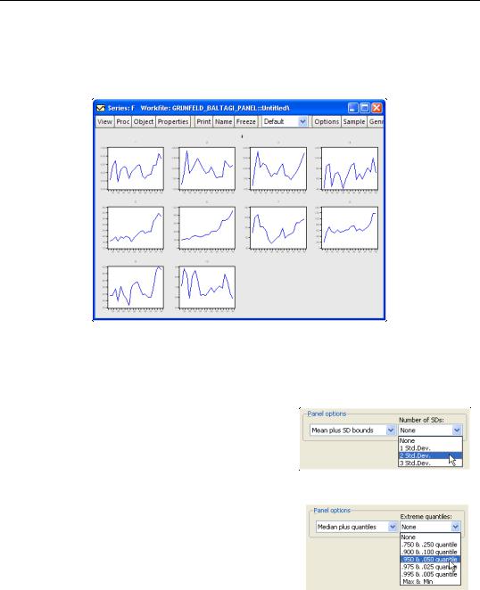
Alternately, selecting Individual cross sections displays separate time series graphs for each cross-section, while Combined cross sections displays separate lines for each cross-
Basic Panel Analysis—637
section in a single graph. We caution you that both types of panel graphs may become difficult to read when there are large numbers of cross-sections. For example, the individual graphs for the 10 cross-section panel data depicted here provide information on general trends, but little in the way of detail:
Nevertheless, the graph does offer you the ability examine all of your cross-sections at-a- glance.
The remaining two options allow you to plot a single graph containing summary statistics for each period.
For line graphs, you may select Mean plus SD bounds, and then use the drop down menu on the lower right to choose between displaying no bounds, and 1, 2, or 3 standard deviation bounds. For other graph types such as area or spike, you may only display the means of the data by period.
For line graphs you may select Median plus quantiles, and then use the drop down menu to choose additional extreme quantiles to be displayed. For other graph types, only the median may be plotted.
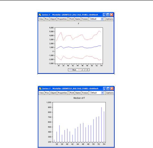
Suppose, for example, that we display a line graph containing the mean and 2 standard deviation
bounds for the F series. EViews computes, for each period, the mean and standard deviation of F across cross-sections, and displays these in a time series graph:
638—Chapter 36. Working with Panel Data
Similarly, we may display a spike graph of the medians of F for each period:
Displaying graph views of a group object in a panel workfile involves similar choices about the handling of the panel structure.
Panel Unit Root Tests
EViews provides convenient tools for computing panel unit root tests. You may compute one or more of the following tests: Levin, Lin and Chu (2002), Breitung (2000), Im, Pesaran and Shin (2003), Fisher-type tests using ADF and PP tests—Maddala and Wu (1999), Choi (2001), and Hadri (2000).
These tests are described in detail in “Panel Unit Root Test,” beginning on page 391.
Basic Panel Analysis—639
To compute the unit root test on a series, simply select View/ Unit Root Test…from the menu of a series object.
By default, EViews will compute a Summary of all of the first five unit root tests, where applicable, but you may use the combo box in the upper left hand corner to select an individual test statistic.
In addition, you may use the dialog to specify trend and intercept settings, to specify lag length selection, and to pro-
vide details on the spectral estimation used in computing the test statistic or statistics.
To begin, we open the F series in our example panel workfile, and accept the defaults to compute the summary of several unit root tests on the level of F. The results are given by
Panel unit root test: Summary
Date: 08/22/06 Time: 17:05
Sample: 1935 1954
Exogenous variables: Individual effects
User specified lags at: 1
Newey-West bandwidth selection using Bartlett kernel
Balanced observations for each test
Cross-
Method
Statistic
Prob.**
sections
Obs
Null: Unit root (assumes common unit root process)
Levin, Lin & Chu t*
1.71727
0.9570
10
180
Null: Unit root (assumes individual unit root process)
Im, Pesaran and Shin W-stat
-0.51923
0.3018
10
180
ADF - Fisher Chi-square
33.1797
0.0322
10
180
PP - Fisher Chi-square
41.9742
0.0028
10
190
** Probabilities for Fisher tests are computed using an asympotic Chi -square distribution. All other tests assume asymptotic normality.
Note that there is a fair amount of disagreement in these results as to whether F has a unit root, even within tests that evaluate the same null hypothesis (e.g., Im, Pesaran and Shin vs. the Fisher ADF and PP tests).
640—Chapter 36. Working with Panel Data
To obtain additional information about intermediate results, we may rerun the panel unit root procedure, this time choosing a specific test statistic. Computing the results for the IPS test, for example, displays (in addition to the previous IPS results) ADF test statistic results for each cross-section in the panel:
Intermediate ADF test results
Cross
Max
section
t-Stat
Prob.
E(t)
E(Var)
Lag
Lag
Obs
1
-2.3596
0.1659
-1.511
0.953
1
1
18
2
-3.6967
0.0138
-1.511
0.953
1
1
18
3
-2.1030
0.2456
-1.511
0.953
1
1
18
4
-3.3293
0.0287
-1.511
0.953
1
1
18
5
0.0597
0.9527
-1.511
0.953
1
1
18
6
1.8743
0.9994
-1.511
0.953
1
1
18
7
-1.8108
0.3636
-1.511
0.953
1
1
18
8
-0.5541
0.8581
-1.511
0.953
1
1
18
9
-1.3223
0.5956
-1.511
0.953
1
1
18
10
-3.4695
0.0218
-1.511
0.953
1
1
18
Average
-1.6711
-1.511
0.953
Panel Cointegration Tests
EViews provides a number of procedures for computing panel cointegration tests. The following tests are available in EViews: Pedroni (1999, 2004), Kao (1999) and Fisher-type test using Johansen’s test methodology (Maddala and Wu (1999)). The details of these tests are described in “Panel Cointegration Details,” beginning on page 700.
To compute a panel cointegration test, select View/Cointegration Test/Panel Cointegration Test… from the menu of an EViews group. You may use various options for specifying the trend specification, lag length selection and spectral estimation methods.
To illustrate, we perform a Pedroni panel cointegration test. The only modification from the default settings that we make is to select Automatic selection for lag length. Click on OK to accept the settings and perform the test.
Basic Panel Analysis—641
Pedroni Residual Cointegration Test Series: IVM MM
Date: 12/13/06 Time: 11:43
Sample: 1968M01 1995M12 Included observations: 2688 Cross-sections included: 8
Null Hypothesis: No cointegration
Trend assumption: No deterministic trend
Lag selection: Automatic SIC with a max lag of 16 Newey-West bandwidth selection with Bartlett kernel
Alternative hypothesis: common AR coefs. (within-dimension)
Weighted
Statistic
Prob.
Statistic
Prob.
Panel v-Statistic
4.219500
0.0001
4.119485
0.0001
Panel rho-Statistic
-0.400152
0.3682
-2.543473
0.0157
Panel PP-Statistic
0.671083
0.3185
-1.254923
0.1815
Panel ADF-Statistic
-0.216806
0.3897
0.172158
0.3931
Alternative hypothesis: individual AR coefs. (between-dimension)
Statistic
Prob.
Group rho-Statistic
-1.776207
0.0824
Group PP-Statistic
-0.824320
0.2840
Group ADF-Statistic
0.538943
0.3450
The top portion of the output indicates the type of test, null hypothesis, exogenous variables, and other test options. The next section provides several Pedroni panel cointegration test statistics which evaluate the null against both the homogeneous and the heterogeneous alternatives. In this case, eight of the eleven statistics do not reject the null hypothesis of no cointegration at the conventional size of 0.05.
The bottom portion of the table reports auxiliary cross-section results showing intermediate calculating used in forming the statistics. For the Pedroni test this section is split into two sections. The first section contains the Phillips-Perron non-parametric results, and the second section presents the Augmented Dickey-Fuller parametric results.
642—Chapter 36. Working with Panel Data
Cross section specific results
Phillips-Peron results (non-parametric)
Cross ID
AR(1)
Variance
HAC
Bandwidth
Obs
AUT
0.959
54057.16
46699.67
23.00
321
BUS
0.959
98387.47
98024.05
7.00
321
CON
0.966
144092.9
125609.0
4.00
321
CST
0.933
579515.0
468780.9
6.00
321
DEP
0.908
896700.4
572964.8
7.00
321
HOA
0.941
146702.7
165065.5
6.00
321
MAE
0.975
2996615.
2018633.
3.00
321
MIS
0.991
2775962.
3950850.
7.00
321
Augmented Dickey-Fuller results (parametric)
Cross ID
AR(1)
Variance
Lag
Max lag
Obs
AUT
0.983
48285.07
5
16
316
BUS
0.971
95843.74
1
16
320
CON
0.966
144092.9
0
16
321
CST
0.949
556149.1
1
16
320
DEP
0.974
647340.5
2
16
319
HOA
0.941
146702.7
0
16
321
MAE
0.976
2459970.
6
16
315
MIS
0.977
2605046.
3
16
318
In addition, if your sample consists of a single cross-section, you may perform a cointegration test on the single cross-section using the general tools described in Chapter 38. “Cointegration Testing,” on page 685. Simply select View/Cointegration Test/Individual Johansen Cointegration Test… or View/Cointegration Test/Individual Single-Equation Cointegration Test… to compute the appropriate test. Both of these methods will generate an error message if your sample contains more than one cross-section.
Estimation
EViews provides sophisticated tools for estimating equations in your panel structured workfile. See Chapter 37. “Panel Estimation,” beginning on page 647 for documentation.
Stacked By-Group Analysis
There are various by-group analysis tools that may be used to perform analysis of panel data. Previously, we considered an example of using by-group tools to examine data in “Cross-section and Period Summaries” on page 629. Standard by-group views may also be to test for equality of means, medians, or variances between groups, or to examine boxplots by cross-section or period.
Basic Panel Analysis—643
For example, to compute a test of equality of means for F between firms, simply open the series, then select View/Descriptive Statistics & Tests/Equality Tests by Classification....
Enter FN in the Series/Group for Classify edit field, and select OK to continue. EViews will compute and display the results for an ANOVA for F, classifying the data by firm ID. The top portion of the ANOVA results is given by:
Test for Equality of Means of F
Categorized by values of FN
Date: 08/22/06 Time: 17:11
Sample: 1935 1954
Included observations: 200
Method
df
Value
Probability
Anova F-test
(9, 190)
293.4251
0.0000
Welch F-test*
(9, 71.2051)
259.3607
0.0000
*Test allows for unequal cell variances
Analysis of Variance
Source of Variation
df
Sum of Sq.
Mean Sq.
Between
9
3.21E+08
35640052
Within
190
23077815
121462.2
Total
199
3.44E+08
1727831.
Note in this example that we have relatively few cross-sections with moderate numbers of observations in each firm. Data with very large numbers of group identifiers and few observations are not recommended for this type of testing. To test equality of means between periods, call up the dialog and enter either YEAR or DATEID as the series by which you will classify.
644—Chapter 36. Working with Panel Data
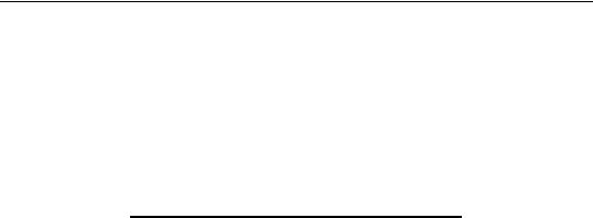
A graphical summary of the primary information in the ANOVA may be obtained by displaying boxplots by cross-section or period. For moderate numbers of distinct classifier values, the graphical display may prove informative. Select View/Graph... to bring up the Graph Options dialog. Select Categorical graph from the drop down on the top left, select Boxplot from the list of graph types, and
enter FN in the Within graph edit field. Click OK to display the boxplots using the default settings.
Stacked Analysis
A wide range of analyses are available in panel structured workfiles that have not been specifically redesigned to use the panel structure of your data. These tools allow you to work with and analyze the stacked data, while taking advantage of the support for handling lags and leads in the panel structured workfile.
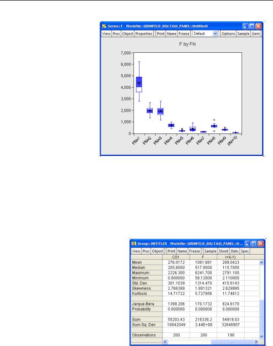
We may, for example, take our example panel workfile, create a group containing the series C01, F, and the expression I+I(-1), and then select View/Descriptive Stats/Individual Samples from the group menu. EViews displays the descriptive statistics for the stacked data.
Note that the calculations are performed over the entire 200 observation stacked data, and that the statistics for I+I(-1) use only 190 observations (200 minus 10 observa-
tions corresponding to the lag of the first observation for each firm).