Panel Workfile Information—619
You may, at any time, click on the Range display line or select Proc/Structure/Resize Current Page... to bring up the Workfile Structure dialog so that you may modify or remove your panel structure.
Observation Labels
The left-hand side of every workfile contains observation labels that identify each observation. In a simple unstructured workfile, these labels are simply the integers from 1 to the total number of observations in the workfile. For dated, non-panel workfiles, these labels are representations of the unique dates associated with each observation. For example, in an annual workfile ranging from 1935 to 1950, the observation labels are of the form “1935”, “1936”, etc.
The observation labels in a panel workfile must reflect the fact that observations possess both cross-section and within-cross-section identifiers. Accordingly, EViews will form observation identifiers using both the cross-section and the cell ID values.
Here, we see the observation labels in an annual panel workfile formed using the cross-section identifiers and a two-digit year identifier.
Panel Workfile Information
When working with panel data, it is important to keep the basic structure of your workfile in mind at all times. EViews provides you with tools to access information about the structure of your workfile.
Workfile Structure
First, the workfile statistics view provides a convenient place for you to examine the structure of your panel workfile. Simply click on View/Statistics from the main menu to display a summary of the structure and contents of your workfile.
620—Chapter 36. Working with Panel Data
Workfile Statistics
Date: 06/17/07 Time: 16:04
Name: GRUNFELD_BALTAGI_PANEL
Number of pages: 1
Page: Untitled |
|
|
|
Workfile structure: Panel - Annual |
|
|
Indices: FN x DATEID |
|
|
|
Panel dimension: 10 x 20 |
|
|
|
Range: 1935 1954 x 10 -- |
200 obs |
|
|
Object |
Count |
Data Points |
|
series |
7 |
1400 |
|
coef |
1 |
751 |
|
Total |
8 |
2151 |
The top portion of the display for our first example workfile is depicted above. The statistics view identifies the page as an annual panel workfile that is structured using the identifiers ID and DATE. There are 10 cross-sections with 20 observations each, for years ranging from 1935 to 1954. For unbalanced data, the number of observations per cross-section reported will be the largest number observed across the cross-sections.
To return the display to the original workfile directory, select View/Workfile Directory from the main workfile menu.
Identifier Indices
EViews provides series expressions and functions that provide information about the crosssection, cell, and observation IDs associated with each observation in a panel workfile.
Cross-section Index
The series expression @crossid provides index identifiers for each observation corresponding to the cross-section to which the observation belongs. If, for example, there are 8 observations with cross-section identifier alpha series values (in order), “B”, “A”, “A”, “A”, “B”, “A”, “A”, and “B”, the command:
series cxid = @crossid
assigns a group identifier value of 1 or 2 to each observation in the workfile. Since the panel workfile is sorted by the cross-section ID values, observations with the identifier value “A” will be assigned a CXID value of 1, while “B” will be assigned 2.
A one-way tabulation of the CXID series shows the number of observations in each crosssection or group:
Panel Workfile Information—621
Tabulation of CXID |
|
|
|
Date: 02/04/04 |
Time: 09:08 |
|
|
|
Sample: 1 8 |
|
|
|
|
Included observations: 8 |
|
|
|
Number of categories: 2 |
|
|
|
|
|
|
|
|
|
|
|
|
|
|
|
|
Cumulative |
Cumulative |
Value |
Count |
Percent |
Count |
Percent |
1 |
5 |
62.50 |
5 |
62.50 |
2 |
3 |
37.50 |
8 |
100.00 |
Total |
8 |
100.00 |
8 |
100.00 |
|
|
|
|
|
|
|
|
|
|
Cell Index
Similarly, @cellid may be used to obtain integers uniquely indexing cell IDs. @cellid numbers observations using an index corresponding to the ordered unique values of the cell or date ID values. Note that since the indexing uses all unique values of the cell or date ID series, the observations within a cross-section may be indexed non-sequentially.
Suppose, for example, we have a panel workfile with two cross-sections. There are 5 observations in the cross-section “A” with cell ID values “1991”, “1992”, “1993”, “1994”, and “1999”, and 3 observations in the cross-section “B” with cell ID values “1993”, “1996”, “1998”. There are 7 unique cell ID values (“1991”, “1992”, “1993”, “1994”, “1996”, “1998”, “1999”) in the workfile.
The series assignment
series cellid = @cellid
will assign to the “A” observations in CELLID the values “1991”, “1992”, “1993”, “1994”, “1997”, and to the “B” observations the values “1993”, “1995”, and “1996”.
A one-way tabulation of the CELLID series provides you with information about the number of observations with each index value:
622—Chapter 36. Working with Panel Data
Tabulation of CELLID |
|
|
|
Date: 02/04/04 |
Time: 09:11 |
|
|
|
Sample: 1 8 |
|
|
|
|
Included observations: 8 |
|
|
|
Number of categories: 7 |
|
|
|
|
|
|
|
|
|
|
|
|
|
|
|
|
Cumulative |
Cumulative |
Value |
Count |
Percent |
Count |
Percent |
1 |
1 |
12.50 |
1 |
12.50 |
2 |
1 |
12.50 |
2 |
25.00 |
3 |
2 |
25.00 |
4 |
50.00 |
4 |
1 |
12.50 |
5 |
62.50 |
5 |
1 |
12.50 |
6 |
75.00 |
6 |
1 |
12.50 |
7 |
87.50 |
7 |
1 |
12.50 |
8 |
100.00 |
Total |
8 |
100.00 |
8 |
100.00 |
|
|
|
|
|
|
|
|
|
|
Within Cross-section Observation Index
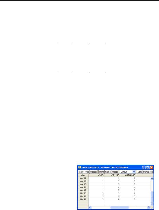
Alternately, @obsid returns an integer uniquely indexing observations within a cross-sec- tion. The observations will be numbered sequentially from 1 through the number of observations in the corresponding cross-section. In the example above, with two cross-section groups “A” and “B” containing 5 and 3 observations, respectively, the command:
series cxid = @crossid
series withinid = @obsid
would number the 5 observations in cross-section “A” from 1 through 5, and the 3 observations in group “B” from 1 through 3.
Bear in mind that while @cellid uses information about all of the ID values in creating its index, @obsid only uses the ordered observations within a cross-section in forming the index. As a result, the only similarity between observations that share an @obsid value is their ordering within the cross-section. In contrast, observations that share a @cellid value also share values for the underlying cell ID.
It is worth noting that if a panel workfile is balanced so that each cross-sec- tion has the same cell ID values, @obsid and @cellid yield identical results.
Workfile Observation Index
In rare cases, you may wish to enumerate the observations beginning at