
- •Preface
- •Part IV. Basic Single Equation Analysis
- •Chapter 18. Basic Regression Analysis
- •Equation Objects
- •Specifying an Equation in EViews
- •Estimating an Equation in EViews
- •Equation Output
- •Working with Equations
- •Estimation Problems
- •References
- •Chapter 19. Additional Regression Tools
- •Special Equation Expressions
- •Robust Standard Errors
- •Weighted Least Squares
- •Nonlinear Least Squares
- •Stepwise Least Squares Regression
- •References
- •Chapter 20. Instrumental Variables and GMM
- •Background
- •Two-stage Least Squares
- •Nonlinear Two-stage Least Squares
- •Limited Information Maximum Likelihood and K-Class Estimation
- •Generalized Method of Moments
- •IV Diagnostics and Tests
- •References
- •Chapter 21. Time Series Regression
- •Serial Correlation Theory
- •Testing for Serial Correlation
- •Estimating AR Models
- •ARIMA Theory
- •Estimating ARIMA Models
- •ARMA Equation Diagnostics
- •References
- •Chapter 22. Forecasting from an Equation
- •Forecasting from Equations in EViews
- •An Illustration
- •Forecast Basics
- •Forecasts with Lagged Dependent Variables
- •Forecasting with ARMA Errors
- •Forecasting from Equations with Expressions
- •Forecasting with Nonlinear and PDL Specifications
- •References
- •Chapter 23. Specification and Diagnostic Tests
- •Background
- •Coefficient Diagnostics
- •Residual Diagnostics
- •Stability Diagnostics
- •Applications
- •References
- •Part V. Advanced Single Equation Analysis
- •Chapter 24. ARCH and GARCH Estimation
- •Basic ARCH Specifications
- •Estimating ARCH Models in EViews
- •Working with ARCH Models
- •Additional ARCH Models
- •Examples
- •References
- •Chapter 25. Cointegrating Regression
- •Background
- •Estimating a Cointegrating Regression
- •Testing for Cointegration
- •Working with an Equation
- •References
- •Binary Dependent Variable Models
- •Ordered Dependent Variable Models
- •Censored Regression Models
- •Truncated Regression Models
- •Count Models
- •Technical Notes
- •References
- •Chapter 27. Generalized Linear Models
- •Overview
- •How to Estimate a GLM in EViews
- •Examples
- •Working with a GLM Equation
- •Technical Details
- •References
- •Chapter 28. Quantile Regression
- •Estimating Quantile Regression in EViews
- •Views and Procedures
- •Background
- •References
- •Chapter 29. The Log Likelihood (LogL) Object
- •Overview
- •Specification
- •Estimation
- •LogL Views
- •LogL Procs
- •Troubleshooting
- •Limitations
- •Examples
- •References
- •Part VI. Advanced Univariate Analysis
- •Chapter 30. Univariate Time Series Analysis
- •Unit Root Testing
- •Panel Unit Root Test
- •Variance Ratio Test
- •BDS Independence Test
- •References
- •Part VII. Multiple Equation Analysis
- •Chapter 31. System Estimation
- •Background
- •System Estimation Methods
- •How to Create and Specify a System
- •Working With Systems
- •Technical Discussion
- •References
- •Vector Autoregressions (VARs)
- •Estimating a VAR in EViews
- •VAR Estimation Output
- •Views and Procs of a VAR
- •Structural (Identified) VARs
- •Vector Error Correction (VEC) Models
- •A Note on Version Compatibility
- •References
- •Chapter 33. State Space Models and the Kalman Filter
- •Background
- •Specifying a State Space Model in EViews
- •Working with the State Space
- •Converting from Version 3 Sspace
- •Technical Discussion
- •References
- •Chapter 34. Models
- •Overview
- •An Example Model
- •Building a Model
- •Working with the Model Structure
- •Specifying Scenarios
- •Using Add Factors
- •Solving the Model
- •Working with the Model Data
- •References
- •Part VIII. Panel and Pooled Data
- •Chapter 35. Pooled Time Series, Cross-Section Data
- •The Pool Workfile
- •The Pool Object
- •Pooled Data
- •Setting up a Pool Workfile
- •Working with Pooled Data
- •Pooled Estimation
- •References
- •Chapter 36. Working with Panel Data
- •Structuring a Panel Workfile
- •Panel Workfile Display
- •Panel Workfile Information
- •Working with Panel Data
- •Basic Panel Analysis
- •References
- •Chapter 37. Panel Estimation
- •Estimating a Panel Equation
- •Panel Estimation Examples
- •Panel Equation Testing
- •Estimation Background
- •References
- •Part IX. Advanced Multivariate Analysis
- •Chapter 38. Cointegration Testing
- •Johansen Cointegration Test
- •Single-Equation Cointegration Tests
- •Panel Cointegration Testing
- •References
- •Chapter 39. Factor Analysis
- •Creating a Factor Object
- •Rotating Factors
- •Estimating Scores
- •Factor Views
- •Factor Procedures
- •Factor Data Members
- •An Example
- •Background
- •References
- •Appendix B. Estimation and Solution Options
- •Setting Estimation Options
- •Optimization Algorithms
- •Nonlinear Equation Solution Methods
- •References
- •Appendix C. Gradients and Derivatives
- •Gradients
- •Derivatives
- •References
- •Appendix D. Information Criteria
- •Definitions
- •Using Information Criteria as a Guide to Model Selection
- •References
- •Appendix E. Long-run Covariance Estimation
- •Technical Discussion
- •Kernel Function Properties
- •References
- •Index
- •Symbols
- •Numerics

Chapter 36. Working with Panel Data
EViews provides you with specialized tools for working with stacked data that have a panel structure. You may have, for example, data for various individuals or countries that are stacked one on top of another.
The first step in working with stacked panel data is to describe the panel structure of your data: we term this step structuring the workfile. Once your workfile is structured as a panel workfile, you may take advantage of the EViews tools for working with panel data, and for estimating equation specifications using the panel structure.
The following discussion assumes that you have an understanding of the basics of panel data. “Panel Data,” beginning on page 216 of User’s Guide I provides background on the characteristics of panel structured data.
We first review briefly the process of applying a panel structure to a workfile. The remainder of the discussion in this chapter focuses on the basics working with data in a panel workfile. Chapter 37. “Panel Estimation,” on page 647 outlines the features of equation estimation in a panel workfile.
Structuring a Panel Workfile
The first step in panel data analysis is to define the panel structure of your data. By defining a panel structure for your data, you perform the dual tasks of identifying the cross-section associated with each observation in your stacked data, and of defining the way that lags and leads operate in your workfile.
While the procedures for structuring a panel workfile outlined below are described in greater detail elsewhere, an abbreviated review may prove useful (for additional detail, see “Describing a Balanced Panel Workfile” on page 38, “Dated Panels” on page 230, and “Undated Panels” on page 235 of User’s Guide I).

616—Chapter 36. Working with Panel Data
There are two basic ways to create a panel structured workfile. First, you may create a new workfile that has a simple balanced panel structure. Simply select File/New/ Workfile... from the main EViews menu to open the Workfile Create dialog. Next, select Balanced Panel from the Workfile structure type combo box, and fill out the dialog as desired. Here, we create a balanced quarterly panel (ranging from 1970Q1 to 2020Q4) with 200 cross-sections. We also enter “Quarterly” in the Page name edit field.
When you click on OK, EViews will create an appropriately structured workfile with 40,800 observations (51 years, 4 quarters, 200 cross-sections). You may then enter or import the data into the workfile.
More commonly, you will use the second method of structuring a panel workfile, in which you first read stacked data into an unstructured workfile, and then apply a structure to the workfile. While
there are a number of issues involved with this operation, let us consider a simple, illustrative example of the basic method.

Structuring a Panel Workfile—617
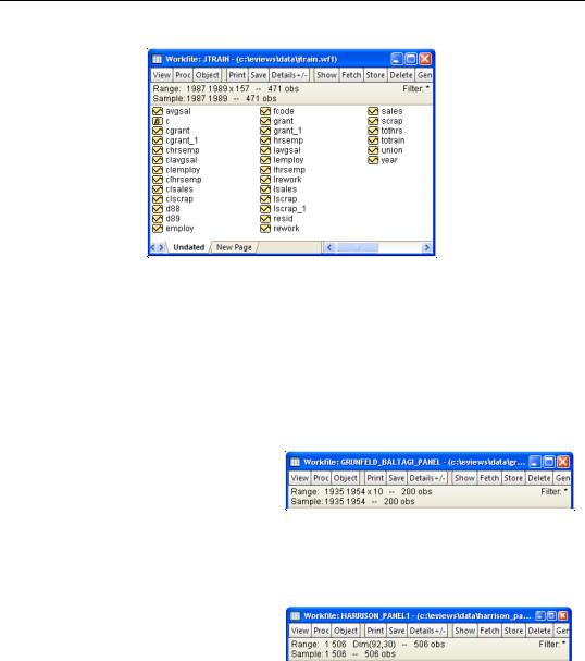
Suppose that we have data for the job training example considered by Wooldridge (2002), using data from Holzer, et al. (1993), which are provided in “Jtrain.WF1”.
These data form a balanced panel of 3 annual observations on 157 firms. The data are first read into a 471 observation, unstructured EViews workfile. The values of the series YEAR and FCODE may be used to identify the date and cross-section, respectively, for each observation.
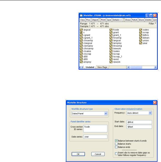
To apply a panel structure to this workfile, simply double click on the “Range:” line at the top of the workfile window, or select Proc/Structure/Resize Current Page... to open the
Workfile structure dialog. Select Dated Panel as our Workfile structure type.
Next, enter YEAR as the Date series and FCODE as the
Cross-section ID series. Since our data form a simple balanced dated panel, we need not concern ourselves with the remaining settings, so we may simply click on OK.
EViews will analyze the data in the specified Date series and Cross-section ID series to determine the appropriate structure for the workfile. The
data in the workfile will be sorted by cross-section ID series, and then by date, and the panel structure will be applied to the workfile.

618—Chapter 36. Working with Panel Data
Panel Workfile Display
The two most prominent visual changes in a panel structured workfile are the change in the range and sample information display at the top of the workfile window, and the change in the labels used to identify individual observations.
Range and Sample
The first visual change in a panel structured workfile is in the Range and Sample descriptions at the top of workfile window.
For a dated panel workfile, EViews will list both the earliest and latest observed dates, the number of crosssections, and the total number of unique observations. Here we see the
top portion of an annual workfile with observations from 1935 to 1954 for 10 cross-sections. Note that workfile sample is described using the earliest and latest observed annual frequency dates (“1935 1954”).
In contrast, an undated panel workfile will display an observation range of 1 to the total number of observations.
The panel dimension statement will
indicate the largest number of observations in a cross-section and the number of cross-sec- tions. Here, we have 92 cross-sections containing up to 30 observations, for a total of 506 observations. Note that the workfile sample is described using the raw observation numbers (“1 506”) since there is no notion of a date pair in undated panels.