Pooled Data—569

Object/Copy Selected… in the main workfile toolbar, or right mouse-click and select Object/Copy... and enter the new name

Pooled Data

As noted previously, all of your pooled data will be held in ordinary EViews series. These series can be used in all of the usual ways: they may, among other things, be tabulated, graphed, used to generate new series, or used in estimation. You may also use a pool object to work with sets of the individual series.

There are two classes of series in a pooled workfile: ordinary series and cross-section specific series.

Ordinary Series

An ordinary series is one that has common values across all cross-sections. A single series may be used to hold the data for each variable, and these data may be applied to every cross-section. For example, in a pooled workfile with firm cross-section identifiers, data on overall economic conditions such as GDP or money supply do not vary across firms. You need only create a single series to hold the GDP data, and a single series to hold the money supply variable.

Since ordinary series do not interact with cross-sections, they may be defined without reference to a pool object. Most importantly, there are no naming conventions associated with ordinary series beyond those for ordinary EViews objects.

Cross-section Specific Series

Cross-section specific series are those that have values that differ between cross-sections. A set of these series are required to hold the data for a given variable, with each series corresponding to data for a specific cross-section.

Since cross-section specific series interact with cross-sections, they should be defined in conjunction with the identifiers in pool objects. Suppose, for example, that you have a pool object that contains the identifiers “_USA,” “_KOR,” “_JPN,” and “_UK”, and that you have time series data on GDP for each of the cross-section units. In this setting, you should have a four cross-section specific GDP series in your workfile.

The key to naming your cross-section specific series is to use names that are a combination of a base name and a cross-section identifier. The cross-section identifiers may be embedded at an arbitrary location in the series name, so long as this is done consistently across identifiers.

You may elect to place the identifier at the end of the base name, in which case, you should name your series “GDP_USA,” “GDP_KOR,” “GDP_JPN,” and “GDP_UK”. Alternatively, you may choose to put the section identifiers in front of the name, so that you have the

Setting up a Pool Workfile—571

and to refer to them collectively as the pool series “ASIA_?”. While not particularly difficult to do, this direct approach becomes more cumbersome the greater the number of cross-sec- tion identifiers.

More easily, we may use the special pool series expression:

@ingrp(asia)

to define a special virtual pool series in which each observation takes a 0 or 1 indicator for whether an observation is in the specified group. This expression is equivalent to creating the four cross-section specific series, and referring to them as “ASIA_?”.

We must emphasize that pool series specifiers using the “?” and the @INGRP function may only be used through a pool object, since they have no meaning without a list of cross-sec- tion identifiers. If you attempt to use a pool series outside the context of a pool object, EViews will attempt to interpret the “?” as a wildcard character (see Appendix A. “Wildcards,” on page 559 in the Command and Programming Reference). The result, most often, will be an error message saying that your variable is not defined.

Setting up a Pool Workfile

Your goal in setting up a pool workfile is to obtain a workfile containing individual series for ordinary variables, sets of appropriately named series for the cross-section specific data, and pool objects containing the related sets of identifiers. The workfile should have frequency and range matching the time series dimension of your pooled data.

There are two basic approaches to setting up such a workfile. The direct approach involves first creating an empty workfile with the desired structure, and then importing data into individual series using either standard or pool specific import methods. The indirect approach involves first creating a stacked representation of the data in EViews, and then using EViews built-in reshaping tools to set up a pooled workfile.

Direct Setup

The direct approach to setting up your pool workfile involves three distinct steps: first creating a workfile with the desired time series structure; next, creating one or more pool objects containing the desired cross-section identifiers; and lastly, using pool object tools to import data into individual series in the workfile.

Creating the Workfile and Pool Object

The first step in the direct setup is to create an ordinary EViews workfile structured to match the time series dimension of your data. The range of your workfile should represent the earliest and latest dates or observations you wish to consider for any of the cross-section units.

Setting up a Pool Workfile—573

multiple columns of unstacked source data. You may read unstacked data directly into EViews using the standard workfile creation procedures described in “Creating a Workfile by Reading from a Foreign Data Source” on page 39 of User’s Guide I. Each cross-section specific variable should be read as an individual series, with the names of the resulting series follow the pool naming conventions given in your pool object. Ordinary series may be imported in the usual fashion with no additional complications.

In this example, we should use the standard EViews tools to read separate series for each column. We create the individual series “YEAR”, “C_USA”, “C_KOR”, “C_JPN”, “G_USA”, “G_JPN”, and “G_KOR”.

Stacked Data

Pooled data can also be arranged in stacked form, where all of the data for a variable are grouped together in a single column.

In the most common form, the data for different cross-sections are stacked on top of one another, with all of the sequentially dated observations for a given cross-section grouped together. We may say that these data are stacked by cross-section:

…… … …

Alternatively, we may have data that are stacked by date, with all of the observations of a given period grouped together:

Setting up a Pool Workfile—575

The indirect method is generally easier to use than the direct approach and has the advantage of not requiring that the stacked data be balanced. It has the disadvantage of using more computer memory since EViews must have two copies of the source data in memory at the same time.

Direct Import of Stacked Data

An alternative approach is to enter or read the data directly into the workfile using a pool object. You may enter or copy-and-paste data from the source into and a stacked representation of your data, or you may use the pool object to describe how to read the stacked data into the unstacked workfile.

To enter data or copy-and-paste, you use the pool object to create a stacked representation of the data in EViews:

•First, specify which time series observations will be included in your stacked spreadsheet by setting the workfile sample.

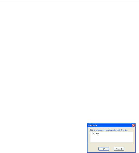
•Next, open the pool, then select View/Spreadsheet View… EViews will prompt you for a list of series. You can enter ordinary series names or pool series names. If the series exist, then EViews will display the data in the series. If the series do not exist, then EViews will create the series or group of series, using the cross-section identifiers if you specify a pool series.

•EViews will open the stacked spreadsheet view of the pool series. If desired, click on the Order +/– button to toggle between stacking by cross-section and stacking by date.

•Click Edit +/– to turn on edit mode in the spreadsheet window, and enter your data, or cut-and-paste from another application.

For example, if we have a pool object that contains the identifiers “_USA”, “_UK”, “_JPN”, and “_KOR”, we can instruct EViews to create the series C_USA, C_UK, C_JPN, C_KOR, and G_USA, G_UK, G_JPN, G_KOR, and YEAR simply by entering the pool series names “C?”, “G?” and the ordinary series name “YEAR”, and pressing OK.

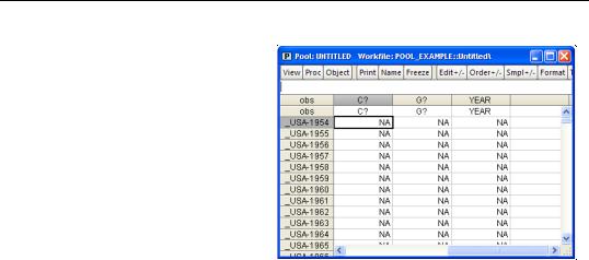
EViews will open a stacked spreadsheet view of the

series in your list. Here we see the series stacked by cross-section, with the pool or ordinary series names in the column header, and the cross-section/date identifiers labeling each row. Note that since YEAR is an ordinary series, its values are repeated for each cross-section in the stacked spreadsheet.

Setting up a Pool Workfile—577

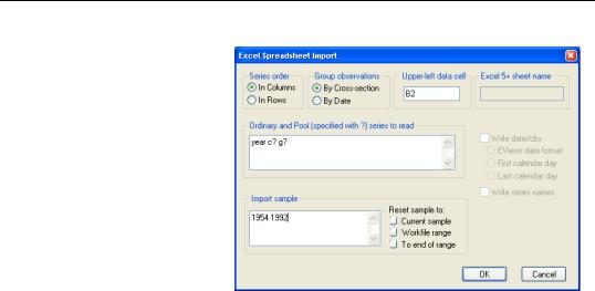
Much of this dialog should be familiar from the discussion in “Importing Data from a Spreadsheet or Text File” on page 105 of User’s Guide I.

First, indicate whether the pool series are in rows or in columns, and whether the data are stacked by crosssection, or stacked by date.

Next, in the pool series edit box, enter the names of the

series you wish to import. This list may contain any combination of ordinary series names and pool series names.

Lastly, fill in the sample information, starting cell location, and optionally, the sheet name.

When you specify your series using pool series names, EViews will, if necessary, create and name the corresponding set of pool series using the list of cross-section identifiers in the pool object. If you list an ordinary series name, EViews will, if needed, create a single series to hold the data.

EViews will read the contents of your file into the specified pool variables using the sample information. When reading into pool series, the first set of observations in the file will be placed in the individual series corresponding to the first cross-section (if reading data that is grouped by cross-section), or the first sample observation of each series in the set of crosssectional series (if reading data that is grouped by date), and so forth.

If you read data into an ordinary series, EViews will continually assign values into the corresponding observation of the single series, so that upon completion of the import procedure, the series will contain the last set of values read from the file.

The basic technique for importing stacked data from ASCII text files is analogous, but the corresponding dialog contains many additional options to handle the complexity of text files.