Working with the State Space—503
reports the maximized log likelihood value, the number of estimated parameters, and the associated information criteria.
Some parts of the output, however, are new and may require discussion. The bottom section provides additional information about the handling of missing values in estimation. “Likelihood observations” reports the actual number of observations that are used in forming the likelihood. This number (which is the one used in computing the information criteria) will differ from the “Included observations” reported at the top of the view when EViews drops an observation from the likelihood calculation because all of the signal equations have missing values. The number of omitted observations is reported in “Missing observations”. “Partial observations” reports the number of observations that are included in the likelihood, but for which some equations have been dropped. “Diffuse priors” indicates the number of initial state covariances for which EViews is unable to solve and for which there is no user initialization. EViews’ handling of initial states and covariances is described in greater detail in “Initial Conditions” on page 509.
EViews also displays the final one-step ahead values of the state vector, aT + 1 T , and the corresponding RMSE values (square roots of the diagonal elements of PT + 1 T ). For settings where you may care about the entire path of the state vector and covariance matrix, EViews provides you with a variety of views and procedures for examining the state results in greater detail.
Working with the State Space
EViews provides a variety of specialized tools for specifying and examining your state space specification. As with other estimation objects, the sspace object provides additional views and procedures for examining the estimation results, performing inference and specification testing, and extracting results into other EViews objects.
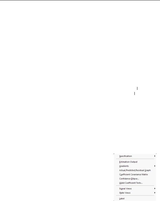
State Space Views
Many of the state space views should be familiar from previous discussion:
•We have already discussed the Specification... views in our analysis of “Specification Views” on page 498.
•The Estimation Output view displays the coefficient estimates and summary statistics as described above in “Interpreting the estimation results” on page 502. You may also access this view by pressing Stats on the sspace toolbar.
•The Gradients and Derivatives... views should be
familiar from other estimation objects. If the sspace contains parameters to be esti-
504—Chapter 33. State Space Models and the Kalman Filter
mated, this view provides summary and visual information about the gradients of the log likelihood at estimated parameters (if the sspace is estimated) or at current parameter values.
•Actual, Predicted, Residual Graph displays, in graphical form, the actual and one-
step ahead fitted values of the signal dependent variable(s), yt t – 1 , and the one-step ahead standardized residuals, et t – 1 .
•Select Coefficient Covariance Matrix to view the estimated coefficient covariance.
•Wald Coefficient Tests… allows you to perform hypothesis tests on the estimated coefficients. For details, see “Wald Test (Coefficient Restrictions)” on page 146.
•Label allows you to annotate your object. See “Labeling Objects” on page 76 of User’s Guide I.
Note that with the exception of the Label and Specification... views, these views are available only following successful estimation of your state space model.
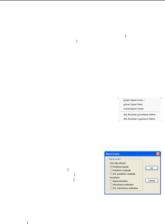
Signal Views
When you click on View/Signal Views, EViews displays a sub-menu containing additional view selections. Two of these selections are always available, even if the state space model has not yet been estimated:
•Actual Signal Table and Actual Signal Graph display
the dependent signal variables in spreadsheet and graphical forms, respectively. If there are multiple signal equations, EViews will display a each series with its own axes.
The remaining views are only available following estimation.
•Graph Signal Series... opens a dialog with choices for the results to be displayed. The dia-
log allows you to choose between the one-step ahead predicted signals, yt t – 1 , the corre-
sponding one-step residuals, et t – 1 , or standardized one-step residuals, et t – 1 , the smoothed signals, yˆ t , smoothed signal distur-
bances, eˆt , or the standardized smoothed signal disturbances, eˆt . ±2 (root mean square) standard error bands are plotted where appro-
priate.
•Std. Residual Correlation Matrix and Std. Residual Covariance Matrix display the correlation and covariance matrix of the standardized one-step ahead signal residual,
Working with the State Space—505
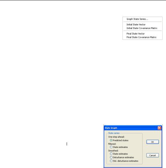
State Views
To examine the unobserved state components, click on View/ State Views to display the state submenu. EViews allows you to examine the initial or final values of the state components, or to graph the full time-path of various filtered or smoothed state data.
Two of the views are available either before or after estimation:
•Initial State Vector and Initial State Covariance Matrix display the values of the initial state vector, a0 , and covariance matrix, P0 . If the unknown parameters have previously been estimated, EViews will evaluate the initial conditions using the esti-
mated values. If the sspace has not been estimated, the current coefficient values will be used in evaluating the initial conditions.
This information is especially relevant in models where EViews is using the current values of the system matrices to solve for the initial conditions. In cases where you are having difficulty starting your estimation, you may wish to examine the values of the initial conditions at the starting parameter values for any sign of problems.
The remainder of the views are only available following successful estimation:
•Final State Vector and Final State Covariance Matrix display the values of the final state vector, aT , and covariance matrix, PT , evaluated at the estimated parameters.
•Select Graph State Series... to display a dialog containing several choices for the state
information. You can graph the one-step ahead predicted states, at t – 1 , the filtered
(contemporaneous) states, at , the smoothed
ˆ
state estimates, at , smoothed state disturbance estimates, vˆt , or the standardized smoothed state disturbances, hˆ t . In each case, the data are displayed along with corresponding ±2 standard error bands.
State Space Procedures
You can use the EViews procedures to create, estimate, forecast, and generate data from your state space specification. Select Proc in the sspace toolbar to display the available procedures:
506—Chapter 33. State Space Models and the Kalman Filter
•Define State Space... calls up the Auto-Specification dialog (see “Auto-Specification” on page 500). This feature provides a method of specifying a variety of common state space specifications using interactive menus.
•Select Estimate... to estimate the parameters of the specification (see “Estimating a State Space Model” on page 501).
These above items are available both before and after estimation. The automatic specification tool will replace the existing state space specification and will clear any results.
Once you have estimated your sspace, EViews provides additional tools for generating data:
•The Forecast... dialog allows you to generate forecasts of the states, signals, and the associated standard errors using alternative methods and initialization approaches.
First, select the forecast method. You can select between dynamic, smoothed, and n-period ahead forecasting, as described in “Forecasting” on page 490. Note that any
lagged endogenous variables on the right-hand side of your signal equations will be treated as predetermined for purposes of forecasting.
EViews allows you to save various types of forecast output in series in your workfile. Simply check any of the output boxes, and specify the names for the series in the corresponding edit field.
You may specify the names either as a list or using a wildcard expression. If you choose to list the names, the number of identifiers must match the number of signals
in your specification. You should be aware that if an output series with a specified name already exists in the workfile, EViews will overwrite the entire contents of the series.
If you use a wildcard expression, EViews will substitute the name of each signal in the appropriate position in the wildcard expression. For example, if you have a model with signals Y1 and Y2, and elect to save the one-step predictions in “PRED*”, EViews will use the series PREDY1 and PREDY2 for output. There are two limitations to this feature: (1) you may not use the wildcard expression “*” to save signal results since this will overwrite the original signal data, and (2) you may not use a wildcard
Working with the State Space—507
when any signal dependent variables are specified by expression, or when there are multiple equations for a signal variable. In both cases, EViews will be unable to create the new series and will generate an error message.
Keep in mind that if your signal dependent variable is an expression, EViews will only provide forecasts of the expression. Thus, if your signal variable is LOG(Y), EViews will forecast the logarithm of Y.
Now enter a sample and specify the treatment of the initial states, and then click OK. EViews will compute the forecast and will place the results in the specified series. No output window will open.
There are several options available for setting the initial conditions. If you wish, you can instruct the sspace object to use the One-step ahead or Smoothed estimates of the state and state covariance as initial values for the forecast period. The two initialization methods differ in the amount of information used from the estimation sample; one-step ahead uses information up to the beginning of the forecast period, while smoothed uses the entire estimation period.
Alternatively, you may use EViews computed initial conditions. As in estimation, if possible, EViews will solve the Algebraic Riccati equations to obtain values for the initial state and state covariance at the start of each forecast interval. If solution of these conditions is not possible, EViews will use diffuse priors for the initial values.
Lastly, you may choose to provide a vector and sym object which contain the values for the forecast initialization. Simply select User Specified and enter the name of valid EViews objects in the appropriate edit fields.
Note that when performing either dynamic or smoothed forecasting, EViews requires that one-step ahead and smoothed initial conditions be computed from the estimation sample. If you choose one of these two forecasting methods and your forecast period begins either before or after the estimation sample, EViews will issue an error and instruct you to select a different initialization method.
When computing n-step ahead forecasting, EViews will adjust the start of the forecast period so that it is possible to obtain initial conditions for each period using the specified method. For the one-step ahead and smoothed methods, this means that at the earliest, the forecast period will begin n – 1 observations into the estimation sample, with earlier forecasted values set to NA. For the other initialization methods, forecast sample endpoint adjustment is not required.
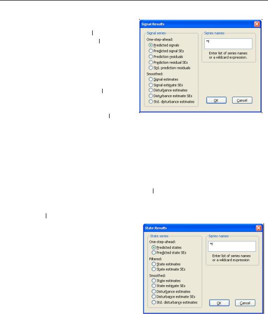
•Make Signal Series... allows you to create series containing various signal results computed over the estimation sample. Simply click on the menu entry to display the results dialog.
508—Chapter 33. State Space Models and the Kalman Filter
You may select the one-step ahead predicted signals, y˜ t t – 1 , one-step prediction residuals, et t – 1 , smoothed signal, yˆ t , or signal disturbance estimates, eˆt . EViews also allows you to save the corresponding standard errors for each of these components (square roots of the diagonal elements of Ft t – 1 , St ,
ˆ
and Qt ), or the standardized values of the one-step residuals and smoothed disturbances, et t – 1 or eˆt .
Next, specify the names of your series in the edit field using a list or wildcards as described above. Click OK to generate a group containing the desired signal series.
As above, if your signal dependent variable is an expression, EViews will only export results based upon the entire expression.
•Make State Series... opens a dialog allowing you to create series containing results
for the state variables computed over the estimation sample. You can choose to save either the one-step ahead state estimate, at t – 1 , the filtered state mean, at , the
smoothed states, aˆ t , state disturbances, vˆt , standardized state disturbances, hˆ t , or the corresponding standard error series (square roots of the diagonal elements of
Pt t – 1 , Pt , Vt and ˆ t ).
Q
Simply select one of the output types, and enter the names of the output series in the edit field. The rules for specifying the output names are the same as for the Forecast... procedure described above. Note that the wildcard expression “*” is permitted when saving state results. EViews will simply use the state names defined in your specification.
We again caution you that if an output series exists in the workfile,
EViews will overwrite the entire contents of the series.
•Click on Make Endogenous Group to create a group object containing the signal dependent variable series.