460—Chapter 32. Vector Autoregression and Error Correction Models
where aij , bij , ci are the parameters to be estimated.
Estimating a VAR in EViews
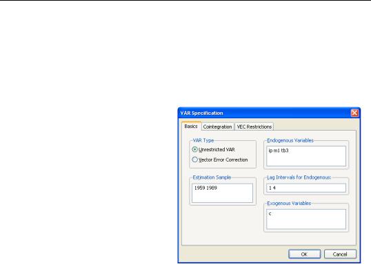
To specify a VAR in EViews, you must first create a var object. Select Quick/Estimate VAR... or type var in the command window. The Basics tab of the VAR Specification dialog will prompt you to define the structure of your VAR.
You should fill out the dialog with the appropriate information:
• Select the VAR type: Unrestricted VAR or Vector Error Correction (VEC). What we have been calling a VAR is actually an unrestricted VAR. VECs are explained below.
• Set the estimation sample.
• Enter the lag specification in the appropriate edit box. This information is entered in pairs: each pair of numbers defines a range of lags. For example, the lag pair shown above:
1 4
tells EViews to use the first through fourth lags of all the endogenous variables in the system as right-hand side variables.
You can add any number of lag intervals, all entered in pairs. The lag specification:
2 4 6 9 12 12
uses lags 2–4, 6–9, and 12.
•Enter the names of endogenous and exogenous series in the appropriate edit boxes. Here we have listed M1, IP, and TB3 as endogenous series, and have used the special series C as the constant exogenous term. If either list of series were longer, we could have created a named group object containing the list and then entered the group name.
The remaining dialog tabs (Cointegration and Restrictions) are relevant only for VEC models and are explained below.
VAR Estimation Output—461
VAR Estimation Output
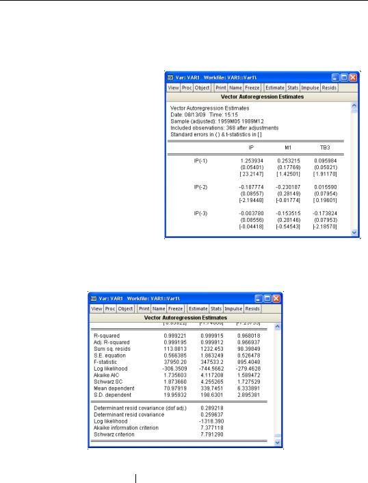
Once you have specified the VAR, click OK. EViews will display the estimation results in the VAR window.
Each column in the table corresponds to an equation in the VAR. For each right-hand side variable, EViews reports the estimated coefficient, its standard error, and the t-statistic. For example, the coefficient for IP(-1) in the TB3 equation is 0.095984.
EViews displays additional information below the coefficient summary. The first part of the additional output presents standard OLS regression statistics for each equation. The results are computed separately for each
equation using the appropriate residuals and are displayed in the corresponding column. The numbers at the very bottom of the table are the summary statistics for the VAR system as a whole.
The determinant of the residual covariance (degree of freedom adjusted) is computed as:
Q
=
1
Âetet
¢
(32.3)
det T – p
ˆ
-------------
ˆ ˆ
t
462—Chapter 32. Vector Autoregression and Error Correction Models
where p is the number of parameters per equation in the VAR. The unadjusted calculation ignores the p . The log likelihood value is computed assuming a multivariate normal (Gaussian) distribution as:
l
=
–
T
{k(1
+ log2p) + log
Q
}
(32.4)
2
---
ˆ
The two information criteria are computed as:
AIC = –2l § T + 2n § T
(32.5)
SC = –2l § T + nlogT § T
where n = k(d + pk) is the total number of estimated parameters in the VAR. These information criteria can be used for model selection such as determining the lag length of the VAR, with smaller values of the information criterion being preferred. It is worth noting that some reference sources may define the AIC/SC differently, either omitting the “inessential” constant terms from the likelihood, or not dividing by T (see also Appendix D. “Information Criteria,” on page 771 for additional discussion of information criteria).
Views and Procs of a VAR
Once you have estimated a VAR, EViews provides various views to work with the estimated VAR. In this section, we discuss views that are specific to VARs. For other views and procedures, see the general discussion of system views in Chapter 31. “System Estimation,” beginning on page 419.
Diagnostic Views
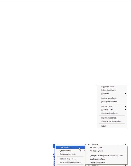
A set of diagnostic views are provided under the menus View/ Lag Structure and View/Residual Tests in the VAR window. These views should help you check the appropriateness of the estimated VAR.
Lag Structure
EViews offers several views for investigating the lag structure of your equation.
AR Roots Table/Graph
Reports the inverse roots of the characteristic AR polynomial; see Lütkepohl (1991). The estimated VAR is stable (stationary) if all roots have
modulus less than one and lie inside the unit circle. If the VAR is not stable, certain results
Views and Procs of a VAR—463
(such as impulse response standard errors) are not valid. There will be kp roots, where k is the number of endogenous variables and p is the largest lag. If you estimated a VEC with r cointegrating relations, k – r roots should be equal to unity.
Pairwise Granger Causality Tests
Carries out pairwise Granger causality tests and tests whether an endogenous variable can be treated as exogenous. For each equation in the VAR, the output displays x2 (Wald) statistics for the joint significance of each of the other lagged endogenous variables in that equation. The statistic in the last row (All) is the x2 statistic for joint significance of all other lagged endogenous variables in the equation.
Warning: if you have estimated a VEC, the lagged variables that are tested for exclusion are only those that are first differenced. The lagged level terms in the cointegrating equations (the error correction terms) are not tested.
Lag Exclusion Tests
Carries out lag exclusion tests for each lag in the VAR. For each lag, the x2 (Wald) statistic for the joint significance of all endogenous variables at that lag is reported for each equation separately and jointly (last column).
Lag Length Criteria
Computes various criteria to select the lag order of an unrestricted VAR. You will be prompted to specify the maximum lag to “test” for. The table displays various information criteria for all lags up to the specified maximum. (If there are no exogenous variables in the VAR, the lag starts at 1; otherwise the lag starts at 0.) The table indicates the selected lag from each column criterion by an asterisk “*”. For columns 4–7, these are the lags with the smallest value of the criterion.
All the criteria are discussed in Lütkepohl (1991, Section 4.3). The sequential modified likelihood ratio (LR) test is carried out as follows. Starting from the maximum lag, test the hypothesis that the coefficients on lag l are jointly zero using the x2 statistics:
LR = (T – m){log
Ql–1
– log
Ql
} ~ x2(k2 )
(32.6)
where m is the number of parameters per equation under the alternative. Note that we employ Sims’ (1980) small sample modification which uses (T – m ) rather than T . We compare the modified LR statistics to the 5% critical values starting from the maximum lag, and decreasing the lag one at a time until we first get a rejection. The alternative lag order from the first rejected test is marked with an asterisk (if no test rejects, the minimum lag will be marked with an asterisk). It is worth emphasizing that even though the individual tests have size 0.05, the overall size of the test will not be 5%; see the discussion in Lütkepohl (1991, p. 125–126).
464—Chapter 32. Vector Autoregression and Error Correction Models
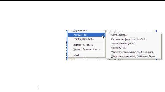
Residual Tests
You may use these views to examine the properties of the residuals from your estimated VAR.
Correlograms
Displays the pairwise crosscorrelograms (sample autocorrelations) for the estimated residuals in the VAR for the specified number of lags. The cross-correlograms
can be displayed in three different formats. There are two tabular forms, one ordered by variables (Tabulate by Variable) and one ordered by lags (Tabulate by Lag). The Graph form displays a matrix of pairwise cross-correlograms. The dotted line in the graphs represent plus or minus two times the asymptotic standard errors of the lagged correlations (computed as 1 § T .
Portmanteau Autocorrelation Test
Computes the multivariate Box-Pierce/Ljung-Box Q-statistics for residual serial correlation up to the specified order (see Lütkepohl, 1991, 4.4.21 & 4.4.23 for details). We report both the Q-statistics and the adjusted Q-statistics (with a small sample correction). Under the null hypothesis of no serial correlation up to lag h , both statistics are approximately distributed x2 with degrees of freedom k2(h – p) where p is the VAR lag order. The asymptotic distribution is approximate in the sense that it requires the MA coefficients to be zero for lags i > h – p . Therefore, this approximation will be poor if the roots of the AR polynomial are close to one and h is small. In fact, the degrees of freedom becomes negative for h < p .
Autocorrelation LM Test
Reports the multivariate LM test statistics for residual serial correlation up to the specified order. The test statistic for lag order h is computed by running an auxiliary regression of the residuals ut on the original right-hand regressors and the lagged residual ut – h , where the missing first h values of ut – h are filled with zeros. See Johansen (1995, p. 22) for the formula of the LM statistic. Under the null hypothesis of no serial correlation of order h , the LM statistic is asymptotically distributed x2 with k2 degrees of freedom.
Normality Test
Reports the multivariate extensions of the Jarque-Bera residual normality test, which compares the third and fourth moments of the residuals to those from the normal distribution. For the multivariate test, you must choose a factorization of the k residuals that are orthogonal to each other (see “Impulse Responses” on page 467 for additional discussion of the need for orthogonalization).
Views and Procs of a VAR—465
Let P
where m3 =
be a k ¥ k factorization matrix such that:
vt = Put ~ N(0, Ik)
(32.7)
ut is the demeaned residuals. Define the third and fourth moment vectors Ât v3t § T and m4 = Ât v4t § T . Then:
m
T
3
6I
k
0
(32.8)
Æ N 0,
m4 – 3
0
24Ik
under the null hypothesis of normal distribution. Since each component is independent of each other, we can form a x2 statistic by summing squares of any of these third and fourth moments.
EViews provides you with choices for the factorization matrix P :
•Cholesky (Lütkepohl 1991, p. 155-158): P is the inverse of the lower triangular Cholesky factor of the residual covariance matrix. The resulting test statistics depend on the ordering of the variables in the VAR.
•Inverse Square Root of Residual Correlation Matrix (Doornik and Hansen 1994):
P = HL–1 / 2H¢V where L is a diagonal matrix containing the eigenvalues of the
residual correlation matrix on the diagonal, H is a matrix whose columns are the corresponding eigenvectors, and V is a diagonal matrix containing the inverse square root of the residual variances on the diagonal. This P is essentially the inverse square root of the residual correlation matrix. The test is invariant to the ordering and to the scale of the variables in the VAR. As suggested by Doornik and Hansen (1994), we perform a small sample correction to the transformed residuals vt before computing the statistics.
•Inverse Square Root of Residual Covariance Matrix (Urzua 1997): P = GD–1 / 2G¢ where D is the diagonal matrix containing the eigenvalues of the residual covariance matrix on the diagonal and G is a matrix whose columns are the corresponding
eigenvectors. This test has a specific alternative, which is the quartic exponential distribution. According to Urzua, this is the “most likely” alternative to the multivariate normal with finite fourth moments since it can approximate the multivariate Pearson
family “as close as needed.” As recommended by Urzua, we make a small sample correction to the transformed residuals vt before computing the statistics. This small sample correction differs from the one used by Doornik and Hansen (1994); see Urzua
(1997, Section D).
•Factorization from Identified (Structural) VAR: P = B–1Awhere A , B are esti-
mated from the structural VAR model. This option is available only if you have estimated the factorization matrices A and B using the structural VAR (see page 471,
below).
466—Chapter 32. Vector Autoregression and Error Correction Models
EViews reports test statistics for each orthogonal component (labeled RESID1, RESID2, and so on) and for the joint test. For individual components, the estimated skewness m3 and kurtosis m4 are reported in the first two columns together with the p-values from the x2(1) distribution (in square brackets). The Jarque-Bera column reports:
m32
+
(m4 – 3)2
(32.9)
T
------6
-----------------------24
with p-values from the x2(2) distribution. Note: in contrast to the Jarque-Bera statistic computed in the series view, this statistic is not computed using a degrees of freedom correction.
For the joint tests, we will generally report:
l3
=
Tm3¢m3 § 6 Æ x2(k)
l4
=
T(m4 – 3)¢(m4 – 3) § 24 Æ x2(k)
(32.10)
l = l3 + l4 Æ x2(2k).
If, however, you choose Urzua’s (1997) test, l will not only use the sum of squares of the “pure” third and fourth moments but will also include the sum of squares of all cross third
and fourth moments. In this case, l is asymptotically distributed as a x2 with k(k + 1)(k + 2)(k + 7) § 24 degrees of freedom.
White Heteroskedasticity Test
These tests are the extension of White’s (1980) test to systems of equations as discussed by Kelejian (1982) and Doornik (1995). The test regression is run by regressing each cross product of the residuals on the cross products of the regressors and testing the joint significance of the regression. The No Cross Terms option uses only the levels and squares of the original regressors, while the With Cross Terms option includes all non-redundant crossproducts of the original regressors in the test equation. The test regression always includes a constant term as a regressor.
The first part of the output displays the joint significance of the regressors excluding the constant term for each test regression. You may think of each test regression as testing the constancy of each element in the residual covariance matrix separately. Under the null of no heteroskedasticity or (no misspecification), the non-constant regressors should not be jointly significant.
The last line of the output table shows the LM chi-square statistics for the joint significance of all regressors in the system of test equations (see Doornik, 1995, for details). The system LM statistic is distributed as a x2 with degrees of freedom mn , where m = k(k + 1) § 2 is the number of cross-products of the residuals in the system and n is the number of the common set of right-hand side variables in the test regression.
Views and Procs of a VAR—467
Cointegration Test
This view performs the Johansen cointegration test for the variables in your VAR. See “Johansen Cointegration Test,” on page 685 for a description of the basic test methodology.
Note that Johansen cointegration tests may also be performed from a Group object, however, tests performed using the latter do not permit you to impose identifying restrictions on the cointegrating vector.
Notes on Comparability
Many of the diagnostic tests given above may be computed “manually” by estimating the VAR using a system object and selecting View/Wald Coefficient Tests... We caution you that the results from the system will not match those from the VAR diagnostic views for various reasons:
•The system object will, in general, use the maximum possible observations for each equation in the system. By contrast, VAR objects force a balanced sample in case there are missing values.
•The estimates of the weighting matrix used in system estimation do not contain a degrees of freedom correction (the residual sums-of-squares are divided by T rather than by T – k ), while the VAR estimates do perform this adjustment. Even though
estimated using comparable specifications and yielding identifiable coefficients, the test statistics from system SUR and the VARs will show small (asymptotically insignificant) differences.
Impulse Responses
A shock to the i-th variable not only directly affects the i-th variable but is also transmitted to all of the other endogenous variables through the dynamic (lag) structure of the VAR. An impulse response function traces the effect of a one-time shock to one of the innovations on current and future values of the endogenous variables.
If the innovations et are contemporaneously uncorrelated, interpretation of the impulse response is straightforward. The i-th innovation ei,t is simply a shock to the i-th endogenous variable yi,t . Innovations, however, are usually correlated, and may be viewed as having a common component which cannot be associated with a specific variable. In order to interpret the impulses, it is common to apply a transformation P to the innovations so that they become uncorrelated:
vt = P et ~ (0, D)
(32.11)
where D is a diagonal covariance matrix. As explained below, EViews provides several options for the choice of P .
468—Chapter 32. Vector Autoregression and Error Correction Models
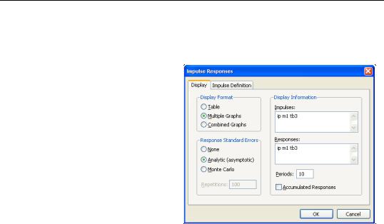
To obtain the impulse response functions, first estimate a VAR. Then select View/Impulse Response... from the VAR toolbar. You will see a dialog box with two tabs: Display and
Impulse Definition.
The Display tab provides the following options:
•Display Format: displays results as a table or graph. Keep in mind that if you choose the Combined Graphs option, the Response Standard Errors option will be ignored and the standard errors will not be displayed. Note also that the output table format is ordered by response variables, not by impulse variables.
•Display Information: you should enter the variables for which you wish to generate innovations (Impulses) and the variables for which you wish to observe the responses (Responses). You may either enter the name of the endogenous variables or the numbers corresponding to the ordering of the variables. For example, if you specified the VAR as GDP, M1, CPI, then you may either type,
GDP CPI M1
or,
1 3 2
The order in which you enter these variables only affects the display of results.
You should also specify a positive integer for the number of periods to trace the response function. To display the accumulated responses, check the Accumulate Response box. For stationary VARs, the impulse responses should die out to zero and the accumulated responses should asymptote to some (non-zero) constant.
•Response Standard Errors: provides options for computing the response standard errors. Note that analytic and/or Monte Carlo standard errors are currently not available for certain Impulse options and for vector error correction (VEC) models. If you choose Monte Carlo standard errors, you should also specify the number of repetitions to use in the appropriate edit box.
If you choose the table format, the estimated standard errors will be reported in parentheses below the responses. If you choose to display the results in multiple
Views and Procs of a VAR—469
graphs, the graph will contain the plus/minus two standard error bands about the impulse responses. The standard error bands are not displayed in combined graphs.
The Impulse tab provides the following options for transforming the impulses:
•Residual—One Unit sets the impulses to one unit of the residuals. This option ignores the units of measurement and the correlations in the VAR residuals so that no transformation is performed. The responses from this option are the MA coefficients of the infinite MA order Wold representation of the VAR.
•Residual—One Std. Dev. sets the impulses to one standard deviation of the residuals. This option ignores the correlations in the VAR residuals.
•Cholesky uses the inverse of the Cholesky factor of the residual covariance matrix to orthogonalize the impulses. This option imposes an ordering of the variables in the VAR and attributes all of the effect of any common component to the variable that comes first in the VAR system. Note that responses can change dramatically if you change the ordering of the variables. You may specify a different VAR ordering by reordering the variables in the Cholesky Ordering edit box.
The (d.f. adjustment) option makes a small sample degrees of freedom correction
when estimating the residual covariance matrix used to derive the Cholesky factor.
The (i,j)-th element of the residual covariance matrix with degrees of freedom correc-
tion is computed as Âtei,t ej,t § (T – p) where p is the number of parameters per equation in the VAR. The (no d.f. adjustment) option estimates the (i,j)-th element
of the residual covariance matrix as Âtei,t ej,t § T . Note: early versions of EViews computed the impulses using the Cholesky factor from the residual covariance matrix
with no degrees of freedom adjustment.
•Generalized Impulses as described by Pesaran and Shin (1998) constructs an orthog-
onal set of innovations that does not depend on the VAR ordering. The generalized impulse responses from an innovation to the j-th variable are derived by applying a variable specific Cholesky factor computed with the j-th variable at the top of the
Cholesky ordering.
•Structural Decomposition uses the orthogonal transformation estimated from the structural factorization matrices. This approach is not available unless you have estimated the structural factorization matrices as explained in “Structural (Identified) VARs” on page 471.
•User Specified allows you to specify your own impulses. Create a matrix (or vector)
that contains the impulses and type the name of that matrix in the edit box. If the VAR has k endogenous variables, the impulse matrix must have k rows and 1 or k
columns, where each column is a impulse vector.
For example, say you have a k = 3 variable VAR and wish to apply simultaneously a positive one unit shock to the first variable and a negative one unit shock to the sec-
470—Chapter 32. Vector Autoregression and Error Correction Models
ond variable. Then you will 1, and 0. Using commands,
matrix(3,1) shock shock.fill(by=c)
create a 3 ¥ 1 impulse matrix containing the values 1, - you can enter:
1,-1,0
and type the name of the matrix SHOCK in the edit box.
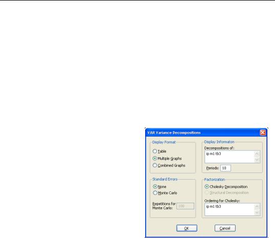
Variance Decomposition
While impulse response functions trace the effects of a shock to one endogenous variable on to the other variables in the VAR, variance decomposition separates the variation in an endogenous variable into the component shocks to the VAR. Thus, the variance decomposition provides information about the relative importance of each random innovation in affecting the variables in the VAR.
To obtain the variance decomposition, select View/Variance Decomposition...
from the var object toolbar. You should provide the same information as for impulse responses above. Note that since non-orthogonal factorization will yield decompositions that do not satisfy an adding up property, your choice of factorization is limited to the Cholesky orthogonal factorizations.
The table format displays a separate variance decomposition for each endogenous variable. The second column, labeled “S.E.”, contains the forecast error of the
variable at the given forecast horizon. The source of this forecast error is the variation in the current and future values of the innovations to each endogenous variable in the VAR. The remaining columns give the percentage of the forecast variance due to each innovation, with each row adding up to 100.
As with the impulse responses, the variance decomposition based on the Cholesky factor can change dramatically if you alter the ordering of the variables in the VAR. For example, the first period decomposition for the first variable in the VAR ordering is completely due to its own innovation.
Factorization based on structural orthogonalization is available only if you have estimated the structural factorization matrices as explained in “Structural (Identified) VARs” on page 471. Note that the forecast standard errors should be identical to those from the Cholesky factorization if the structural VAR is just identified. For over-identified structural VARs, the forecast standard errors may differ in order to maintain the adding up property.