Добавил:
Upload Опубликованный материал нарушает ваши авторские права? Сообщите нам.
Вуз: Предмет: Файл:
Скачиваний:
668
Добавлен:
03.06.2015
Размер:
8.25 Mб
Скачать

402—Chapter 30. Univariate Time Series Analysis

Variance Ratio Test

The question of whether asset prices are predictable has long been the subject of considerable interest. One popular approach to answering this question, the Lo and MacKinlay (1988, 1989) overlapping variance ratio test, examines the predictability of time series data by comparing variances of differences of the data (returns) calculated over different intervals. If we assume the data follow a random walk, the variance of a q -period difference should be q times the variance of the one-period difference. Evaluating the empirical evidence for or against this restriction is the basis of the variance ratio test.

EViews allows you to perform the Lo and MacKinlay variance ratio test for homoskedastic and heteroskedastic random walks, using the asymptotic normal distribution (Lo and MacKinlay, 1988) or wild bootstrap (Kim, 2006) to evaluate statistical significance. In addition, you may compute the rank, rank-score, or sign-based forms of the test (Wright, 2000), with bootstrap evaluation of significance. In addition, EViews offers Wald and multiple comparison variance ratio tests (Richardson and Smith, 1991; Chow and Denning, 1993), so you may perform joint tests of the variance ratio restriction for several intervals.

Performing Variance Ratio Tests in EViews

First, open the series which contains the data which you wish to test and click on View/ Variance Ratio Test… Note that EViews allows you to perform the test using the differences, log differences, or original data in your series as the random walk innovations.

The Output combo determines whether you wish to see your test output in Table or Graph form. (As we discuss below, the choices differ slightly in a panel workfile.)

The Data specification section describes the properties of the data in the series. By default, EViews assumes you wish to test whether the data in the series follow a Random walk, so that variances are computed for differences of the data. Alternately, you may assume that the data fol-

low an Exponential random walk so that the innovations are obtained by taking log differences, or that the series contains the Random walk innovations themselves.

Variance Ratio Test—403

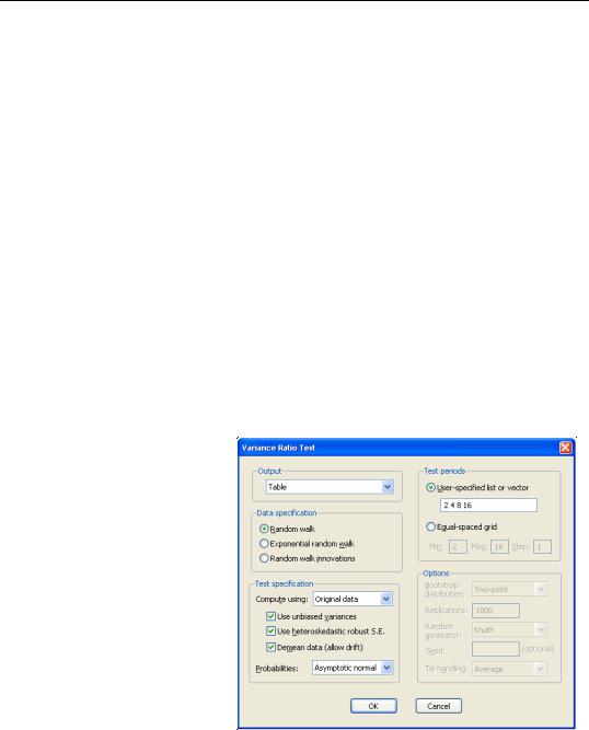
The Test specification section describes the method used to compute your test. By default, EViews computes the basic Lo and MacKinlay variance ratio statistic assuming heteroskedastic increments to the random walk. The default calculations also allow for a non-zero innovation mean and bias correct the variance estimates.

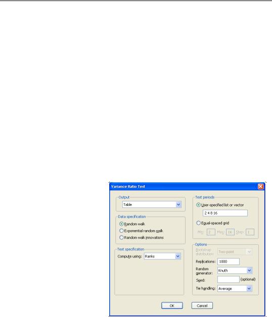
The Compute using combo, which defaults to Original data, instructs EViews to use the original Lo and MacKinlay test statistic based on the innovations obtained from the original data. You may instead use the Compute using combo to instruct EViews to perform the variance ratio test using Ranks, Rank scores (van der Waerden scores), or Signs of the data.

For the Lo and MacKinlay test statistic, the three checkboxes directly beneath the combo allow you to choose whether to bias-correct the variance estimates, to construct the test using the heteroskedasticity robust test standard error, and to allow for non-zero means in the innovations. The Probabilities combo may be used to select between computing the test probabilities using the default Asymptotic normal results (Lo and MacKinlay 1988), or using the Wild bootstrap (Kim 2006). If you choose to perform a wild bootstrap, the Options portion on the lower right of the dialog will prompt you to choose a bootstrap error distribution (Two-point, Rademacher, Normal), number of replications, random number generator, and to specify an optional random number generator seed.

For variance ratio test computed using Ranks, Rank scores (van der Waerden scores), or Signs of the data, the probabilities will be computed by permutation bootstrapping using the settings specified under Options. For the ranks and rank scores tests, there is an additional Tie handling option for the method of assigning ranks in the presence of tied data.

Lastly, the Test periods section identifies the intervals whose variances you wish to compare to the variance of

the one-period innovations. You may specify a single period or more than one period; if there is more than one period, EViews will perform one ore more joint tests of the variance ratio restrictions for the specified periods.

404—Chapter 30. Univariate Time Series Analysis

There are two ways to specify the periods to test. First, you may provide a user-specified list of values or name of a vector containing the values. The default settings, depicted above, are to compute the test for periods “2 4 8 16.” Alternately, you may click on the Equalspaced grid radio, and enter a minimum, maximum, and step.

If you are performing your test on a series in a panel workfile, the Output options differ slightly. If you wish to produce output in tabular form, you can choose to compute individual variance

ratio tests for each cross-section and form a Fisher Combined test (Table - Fisher Combined), or you can choose to stack the cross-sections into a single series and perform the test on the stacked panel (Table - Stacked Panel). Note that the stacked panel method assumes that all means and variances are the same across all cross-sections; the only adjustment for the panel structure is in data handling that insures that lags never cross the seams between cross-sections. There are two graphical counterparts to the table choices: Graph - Individual, which produces a graph for each cross-section, and Graph - Stacked Panel, which produces a graph of the results for the stacked analysis.

An Example

In our example, we employ the time series data on nominal exchange rates used by Wright (2000) to illustrate his modified variance ratio tests (“Wright.WF1”). The data in the first page (WRIGHT) of the workfile provide the relative-to-U.S. exchange rates for the Canadian dollar, French franc, German mark, Japanese yen, and the British pound for the 1,139 weeks from August 1974 through May 1996. Of interest is whether the exchange rate returns, as measured by the log differences of the rates, are i.i.d. or martingale difference, or alternately, whether the exchange rates themselves follow an exponential random walk.

We begin by performing tests on the Japanese yen. Open the JP series, then select

View/Variance Ratio... to display the dialog. We will make a few changes to the default settings to match Wright’s calculations. First, select Exponential random walk in the Data specification section to tell EViews that you wish to work with the log returns. Next, uncheck the Use unbiased variances and Use heteroskedastic robust S.E. check-

Variance Ratio Test—405

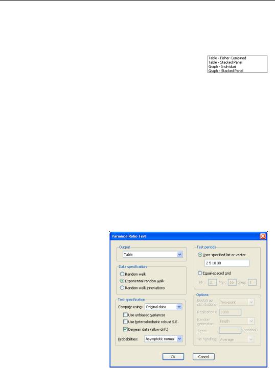
boxes to perform the i.i.d. version of the Lo-MacKinlay test with no bias correction. Lastly, change the user-specified test periods to “2 5 10 30” to match the test periods examined by Wright. Click on OK to compute and display the results.

The top portion of the output shows the test settings and basic test results.

Null Hypothesis: Log JP is a random walk

Date: 04/21/09 Time: 15:15

Sample: 8/07/1974 5/29/1996

Included observations: 1138 (after adjustments)

Standard error estimates assume no heteroskedasticity

Use biased variance estimates

User-specified lags: 2 5 10 30

Joint Tests

Value

df

Probability

Max |z| (at period 5)*

4.295371

1138

0.0001

Wald (Chi-Square)

22.63414

4

0.0001

Individual Tests


Period

Var. Ratio

Std. Error

z-Statistic

Probability

2

1.056126

0.029643

1.893376

0.0583

5

1.278965

0.064946

4.295371

0.0000

10

1.395415

0.100088

3.950676

0.0001

30

1.576815

0.182788

3.155651

0.0016


*Probability approximation using studentized maximum modulus with parameter value 4 and infinite degrees of freedom

Since we have specified more than one test period, there are two sets of test results. The “Joint Tests” are the tests of the joint null hypothesis for all periods, while the “Individual Tests” are the variance ratio tests applied to individual periods. Here, the Chow-Denning maximum z statistic of 4.295 is associated with the period 5 individual test. The approximate p-value of 0.0001 is obtained using the studentized maximum modulus with infinite degrees of freedom so that we strongly reject the null of a random walk. The results are quite similar for the Wald test statistic for the joint hypotheses. The individual statistics generally reject the null hypothesis, though the period 2 variance ratio statistic p-value is slightly greater than 0.05.

The bottom portion of the output shows the intermediate results for the variance ratio test calculations, including the estimated mean, individual variances, and number of observations used in each calculation.

Test Details (Mean = -0.000892835617901)

Period

Variance

Var. Ratio

Obs.

1

0.00021

--

1138

2

0.00022

1.05613

1137

5

0.00027

1.27897

1134

10

0.00029

1.39541

1129

30

0.00033

1.57682

1109


406—Chapter 30. Univariate Time Series Analysis

Alternately, we may display a graph of the test statistics using the same settings. Simply click again on View/Variance Ratio Test..., change the Output combo from Table to

Graph, then fill out the dialog as before and click on OK:

EViews displays a graph of the variance ratio statistics and plus or minus two asymptotic standard error bands, along with a horizontal reference line at 1 representing the null hypothesis. Here, we see a graphical representation of the fact that with the exception of the test against period 2, the null reference line lies outside the bands.

Next, we repeat the previous analysis but allow for heteroskedasticity in the data and use bootstrapping to evaluate the statistical significance. Fill out the dialog as before, but enable the Use heteroskedastic

robust S.E. checkbox and use the Probabilities combo to select Wild bootstrap (with the two-point distribution, 5000 replications, the Knuth generator, and a seed for the random number generator of 1000 specified in the Options section). The top portion of the results is depicted here:

Null Hypothesis: Log JP is a martingale Date: 04/21/09 Time: 15:15

Sample: 8/07/1974 5/29/1996

Included observations: 1138 (after adjustments) Heteroskedasticity robust standard error estimates Use biased variance estimates

User-specified lags: 2 5 10 30

Test probabilities computed using wild bootstrap: dist=twopoint, reps=5000, rng=kn, seed=1000

Joint Tests

Value

df

Probability

Max |z| (at period 5)

3.646683

1138

0.0012

Individual Tests


Period

Var. Ratio

Std. Error

z-Statistic

Probability

2

1.056126

0.037086

1.513412

0.1316

5

1.278965

0.076498

3.646683

0.0004

10

1.395415

0.115533

3.422512

0.0010

30

1.576815

0.205582

2.805766

0.0058


Note that the Wald test is no longer displayed since the test methodology is not consistent with the use of heteroskedastic robust standard errors in the individual tests. The p-values

Variance Ratio Test—407

for the individual variance ratio tests, which are all generated using the wild bootstrap, are generally consistent with the previous results, albeit with probabilities that are slightly higher than before. The individual period 2 test, which was borderline (in)significant in the homoskedastic test, is no longer significant at conventional levels. The Chow-Denning joint test statistic of 3.647 has a bootstrap p-value of 0.0012 and strongly rejects the null hypothesis that the log of JP is a martingale.

Lastly, we perform Wright’s rank variance ratio test with ties replaced by the average of the tied ranks. The test probabilities for this test are computed using the permutation bootstrap, whose settings we select to match those for the previous bootstrap:

Null Hypothesis: Log JP is a random walk Date: 04/21/09 Time: 15:16

Sample: 8/07/1974 5/29/1996

Included observations: 1138 (after adjustments) Standard error estimates assume no heteroskedasticity User-specified lags: 2 5 10 30

Test probabilities computed using permutation bootstrap: reps=5000, rng=kn, seed=1000

Joint Tests

Value

df

Probability

Max |z| (at period 5)

5.415582

1138

0.0000

Wald (Chi-Square)

37.92402

4

0.0000

Individual Tests


Period

Var. Ratio

Std. Error

z-Statistic

Probability

2

1.081907

0.029643

2.763085

0.0050

5

1.351718

0.064946

5.415582

0.0000

10

1.466929

0.100088

4.665193

0.0000

30

1.790412

0.182788

4.324203

0.0000


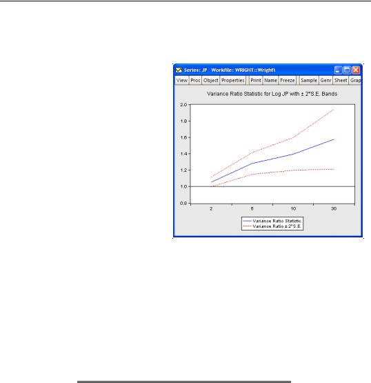
The standard errors employed in forming the individual z-statistics (and those displayed in the corresponding graph view) are obtained from the asymptotic normal results. The probabilities for the individual z-statistics and the joint max z and Wald statistics, which all strongly reject the null hypothesis, are obtained from the permutation bootstrap.

The preceding analysis may be extended to tests that jointly consider all five exchange rates in a panel setting. The second page (WRIGHT_STK) of the “Wright.WF1” workfile contains the panel dataset of the relative-to-U.S. exchange rates described above (Canada, Germany, France, Japan, U.K.). Click on the WRIGHT_STK tab to make the second page active, double click on the EXCHANGE series to open the stacked exchange rates series, then select View/

Variance Ratio Test...

We will redo the heterogeneous Lo and MacKinlay test example from above using the panel data series. Select Table - Fisher Combined in the Output combo then fill out the remainder of the dialog as before, then click on OK. The output, which takes a moment to generate since we are performing 5000 bootstrap replications for each cross-section, consists of two distinct parts. The top portion of the output:

408—Chapter 30. Univariate Time Series Analysis

Null Hypothesis: Log EXCHANGE is a martingale Date: 04/21/09 Time: 15:18

Sample: 8/07/1974 5/29/1996 Cross-sections included: 5

Total panel observations: 5690 (after adjustments) Heteroskedasticity robust standard error estimates Use biased variance estimates

User-specified lags: 2 5 10 30

Test probabilities computed using wild bootstrap: dist=Two-point, reps=5000, rng=kn, seed=1000

Summary Statistics


Statistics


Max |z|

Prob.


df


Fisher Combined


28.252

0.0016


10

shows the test settings and provides the joint Fisher combined test statistic which, in this case, strongly rejects the joint null hypothesis that all of the cross-sections are martingales.

The bottom portion of the output:

Cross-section Joint Tests


Cross-section


Max |z|

Prob.


Obs.


CAN


2.0413

0.0952


1138

DEU


1.7230

0.1952


1138

FRA


2.0825

0.0946


1138

JP


3.6467

0.0016


1138

UK


1.5670

0.2606


1138


depicts the max z statistics for the individual cross-sections, along with corresponding wild bootstrap probabilities. Note that four of the five individual test statistics do not reject the joint hypothesis at conventional levels. It would therefore appear that the Japanese yen result is the driving force behind the Fisher combined test rejection.

Technical Details

Suppose we have the time series {Yt}

= (Y0, Y1, Y2, º, YT) satisfying


DYt

= m + et

(30.53)

where m is an arbitrary drift parameter. The key properties of a random walk that we would like to test are E(et) = 0 for all t and E(etet j) = 0 for any positive j .

The Basic Test Statistic

Lo and MacKinlay (1988) formulate two test statistics for the random walk properties that are applicable under different sets of null hypothesis assumptions about et :

Variance Ratio Test—409

First, Lo and MacKinlay make the strong assumption that the et are i.i.d. Gaussian with variance j2 (though the normality assumption is not strictly necessary). Lo and MacKinlay term this the homoskedastic random walk hypothesis, though others refer to this as the i.i.d. null.

Alternately, Lo and MacKinlay outline a heteroskedastic random walk hypothesis where they weaken the i.i.d. assumption and allow for fairly general forms of conditional heteroskedasticity and dependence. This hypothesis is sometimes termed the martingale null, since it offers a set of sufficient (but not necessary), conditions for et to be a martingale difference sequence (m.d.s.).

We may define estimators for the mean of first difference and the scaled variance of the q -th difference:


1


T


m

=

T

Â

(Yt Yt – 1 )


ˆ


---


t

= 1


(30.54)


1


T


2


2

j

(q) =


Â

(Yt

Yt q qm)


Tq


ˆ


------


ˆ


t = 1


and the corresponding variance ratio VR(q) =

ˆ 2

ˆ

2

(1). The variance estimators

j

(q) § j


may be adjusted for bias, as suggested by Lo and MacKinlay, by replacing T in

Equation (30.54) with (T q + 1)

in the no-drift case, or with (T q + 1)(1 – q § T) in

the drift case.

Lo and MacKinlay show that the variance ratio z-statistic:


z(q)


ˆ2

(q)]

–1 § 2


(30.55)


= (VR(q) – 1) [s


ˆ

2

(q).


is asymptotically N(0, 1) for appropriate choice of estimator s


Under the i.i.d. hypothesis we have the estimator,


ˆ

2

(q) =


2(2q – 1)(q – 1)


(30.56)


s


-----------------------------------------


3qT


while under the m.d.s. assumption we may use the kernel estimator,


2


q – 1


2(q j)

2


ˆ


(q) =


Â


ˆ


-------------------

dj


(30.57)


s


q


j = 1


where


ˆ


T


2


2

T


ˆ 2 2


dj


Â

(yt

j mˆ )


(yt

mˆ )


Â

(yt j

m)


(30.58)

=


§


t = j + 1


t = j + 1


410—Chapter 30. Univariate Time Series Analysis

Joint Variance Ratio Tests

Since the variance ratio restriction holds for every difference q > 1 , it is common to evaluate the statistic at several selected values of q .

To control the size of the joint test, Chow and Denning (1993) propose a (conservative) test statistic that examines the maximum absolute value of a set of multiple variance ratio statistics. The p-value for the Chow-Denning statistic using m variance ratio statistics is bounded from above by the probability for the Studentized Maximum Modulus (SMM) distribution with parameter m and T degrees-of-freedom. Following Chow and Denning, we approximate this bound using the asymptotic (T = •) SMM distribution.

An second approach is available for variance ratio tests of the i.i.d. null. Under this set of assumptions, we may form the joint covariance matrix of the variance ratio test statistics as in Richardson and Smith (1991), and compute the standard Wald statistic for the joint hypothesis that all m variance ratio statistics equal 1. Under the null, the Wald statistic is asymptotic Chi-square with m degrees-of-freedom.

For a detailed discussion of these tests, see Fong, Koh, and Ouliaris (1997).

Wild Bootstrap

Kim (2006) offers a wild bootstrap approach to improving the small sample properties of variance ratio tests. The approach involves computing the individual (Lo and MacKinlay) and joint (Chow and Denning, Wald) variance ratio test statistics on samples of T observations formed by weighting the original data by mean 0 and variance 1 random variables, and using the results to form bootstrap distributions of the test statistics. The bootstrap p- values are computed directly from the fraction of replications falling outside the bounds defined by the estimated statistic.

EViews offers three distributions for constructing wild bootstrap weights: the two-point, the Rademacher, and the normal. Kim’s simulations indicate that the test results are generally insensitive to the choice of wild bootstrap distribution.

Rank and Rank Score Tests

Wright (2000) proposes modifying the usual variance ratio tests using standardized ranks of the increments, DYt . Letting r(DYt) be the rank of the DYt among all T values, we define the standardized rank (r1t) and van der Waerden rank scores (r2t ):


=


T + 1

§

(T – 1)(T + 1)


r1t

r(DYt)

-------------2

-------------------------------------12

(30.59)

r2t

=

F–1(r(DYt) § (T + 1))


In cases where there are tied ranks, the denominator in r1t may be modified slightly to account for the tie handling.

Соседние файлы в папке EViews Guides BITCH