362—Chapter 29. The Log Likelihood (LogL) Object
@derivstep(1) @all 1.49e-8 1e-10
where “1” in the parentheses indicates that one-sided numeric derivatives should be used and @all indicates that the following setting applies to all of the parameters. The first number following @all is the relative step size and the second number is the minimum step
size. The default relative step size is set to the square root of machine epsilon (1.49 ¥ 10–8 ) and the minimum step size is set to m = 10–10 .
The step size can be set separately for each parameter in a single or in multiple @derivstep statements. The evaluation method option specified in parentheses is a global option; it cannot be specified separately for each parameter.
For example, if you include the line:
@derivstep(2) c(2) 1e-7 1e-10
the relative step size for coefficient C(2) will be increased to m = 10–7 and a two-sided derivative will be used to evaluate the derivative. In a more complex example,
@derivstep(2) @all 1.49e-8 1e-10 c(2) 1e-7 1e-10 c(3) 1e-5 1e-8
computes two-sided derivatives using the default step sizes for all coefficients except C(2) and C(3). The values for these latter coefficients are specified directly.
Estimation
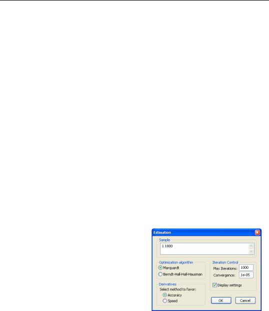
Once you have specified the logl object, you can ask EViews to find the parameter values which maximize the likelihood parameters. Simply click the Estimate button in the likelihood window toolbar to open the Estimation Options dialog.
There are a number of options which allow you to control various aspects of the estimation procedure. See “Setting Estimation Options” on page 751 for a discussion of these options. The default settings, however, should provide a good start for most problems. When you click on OK, EViews will begin estimation using the current settings.
Starting Values
Since EViews uses an iterative algorithm to
find the maximum likelihood estimates, the choice of starting values is important. For problems in which the likelihood function is globally concave, it will influence how many iterations are taken for estimation to converge. For problems where the likelihood function is not concave, it may determine which of several local maxima is found. In some cases, estimation will fail unless reasonable starting values are provided.
Estimation—363
By default, EViews uses the values stored in the coefficient vector or vectors prior to estimation. If a @param statement is included in the specification, the values specified in the statement will be used instead.
In our conditional heteroskedasticity regression example, one choice for starting values for the coefficients of the mean equation coefficients are the simple OLS estimates, since OLS provides consistent point estimates even in the presence of (bounded) heteroskedasticity.
To use the OLS estimates as starting values, first estimate the OLS equation by the command:
equation eq1.ls y c x z
After estimating this equation, the elements C(1), C(2), C(3) of the C coefficient vector will contain the OLS estimates. To set the variance scale parameter C(4) to the estimated OLS residual variance, you can type the assignment statement in the command window:
c(4) = eq1.@se^2
For the final heteroskedasticity parameter C(5), you can use the residuals from the original OLS regression to carry out a second OLS regression, and set the value of C(5) to the appropriate coefficient. Alternatively, you can arbitrarily set the parameter value using a simple assignment statement:
c(5) = 1
Now, if you estimate the logl specification immediately after carrying out the OLS estimation and subsequent commands, it will use the values that you have placed in the C vector as starting values.
As noted above, an alternative method of initializing the parameters to known values is to include a @param statement in the likelihood specification. For example, if you include the line:
@param c(1) 0.1 c(2) 0.1 c(3) 0.1 c(4) 1 c(5) 1
in the specification of the logl, EViews will always set the starting values to C(1)=C(2)=C(3)=0.1, C(4)=C(5)=1.
See also the discussion of starting values in “Starting Coefficient Values” on page 751.
Estimation Sample
EViews uses the sample of observations specified in the Estimation Options dialog when estimating the parameters of the log likelihood. EViews evaluates each expression in the logl for every observation in the sample at current parameter values, using the by observation or by equation ordering. All of these evaluations follow the standard EViews rules for evaluating series expressions.
364—Chapter 29. The Log Likelihood (LogL) Object
If there are missing values in the log likelihood series at the initial parameter values, EViews will issue an error message and the estimation procedure will stop. In contrast to the behavior of other EViews built-in procedures, logl estimation performs no endpoint adjustments or dropping of observations with missing values when estimating the parameters of the model.
LogL Views
•Likelihood Specification: displays the window where you specify and edit the likelihood specification.
•Estimation Output: displays the estimation results obtained from maximizing the likelihood function.
•Covariance Matrix: displays the estimated covariance matrix of the parameter estimates. These are computed from the inverse of the sum of the outer product of the first derivatives evaluated at the optimum parameter values. To save this covariance matrix as a symmetric matrix object, you may use the @coefcov data member.
•Wald Coefficient Tests…: performs the Wald coefficient restriction test. See “Wald Test (Coefficient Restrictions)” on page 146, for a discussion of Wald tests.
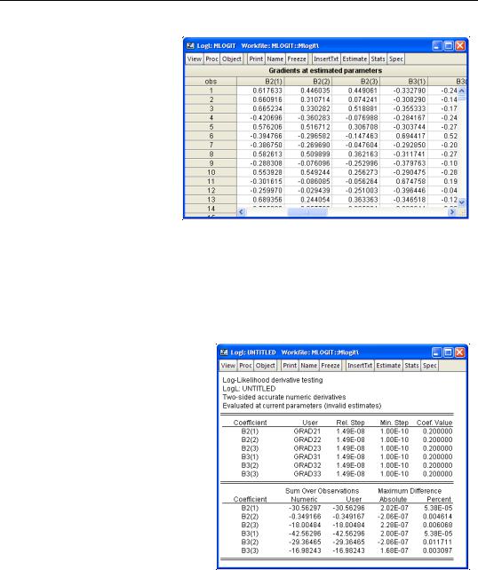
•Gradients: displays view of the gradients (first derivatives) of the log likelihood at the current parameter values (if the model has not yet been estimated), or at the converged parameter values (if the model has been estimated). These views may prove to be useful diagnostic tools if you are experiencing problems with convergence.
•Check Derivatives: displays the values of the numeric derivatives and analytic derivatives (if available) at the starting values (if a @param statement is included), or at current parameter values (if there is no @param statement).
LogL Procs
•Estimate…: brings up a dialog to set estimation options, and to estimate the parameters of the log likelihood.
•Make Model: creates an untitled model object out of the estimated likelihood specification.
•Make Gradient Group: creates an untitled group of the gradients (first derivatives) of the log likelihood at the estimated parameter values. These gradients are often used in constructing Lagrange multiplier tests.
•Update Coefs from LogL: updates the coefficient vector(s) with the estimates from the likelihood object. This procedure allows you to export the maximum likelihood estimates for use as starting values in other estimation problems.
LogL Procs—365
Most of these procedures should be familiar to you from other EViews estimation objects. We describe below the features that are specific to the logl object.
Estimation Output
In addition to the coefficient and standard error estimates, the standard output for the logl object describes the method of estimation, sample used in estimation, date and time that the logl was estimated, evaluation order, and information about the convergence of the estimation procedure.
LogL: MLOGIT
Method: Maximum Likelihood (Marquardt)
Date: 08/12/09 Time: 12:25
Sample: 1 1000
Included observations: 1000
Evaluation order: By equation
Convergence achieved after 8 iterations
|
Coefficient |
Std. Error |
z-Statistic |
Prob. |
|
|
|
|
|
|
|
|
|
|
B2(1) |
-0.521793 |
0.205568 |
-2.538302 |
0.0111 |
B2(2) |
0.994358 |
0.267963 |
3.710798 |
0.0002 |
B2(3) |
0.134983 |
0.265655 |
0.508115 |
0.6114 |
B3(1) |
-0.262307 |
0.207174 |
-1.266122 |
0.2055 |
B3(2) |
0.176770 |
0.274756 |
0.643371 |
0.5200 |
B3(3) |
0.399166 |
0.274056 |
1.456511 |
0.1453 |
|
|
|
|
|
|
|
|
Log likelihood |
-1089.415 |
Akaike info criterion |
2.190830 |
Avg. log likelihood |
-1.089415 |
Schwarz criterion |
2.220277 |
Number of Coefs. |
6 |
Hannan-Quinn criter. |
2.202022 |
|
|
|
|
|
|
|
|
|
|
EViews also provides the log likelihood value, average log likelihood value, number of coefficients, and three Information Criteria. By default, the starting values are not displayed. Here, we have used the Estimation Options dialog to instruct EViews to display the estimation starting values in the output.
Gradients
The gradient summary table and gradient summary graph view allow you to examine the gradients of the likelihood. These gradients are computed at the current parameter values (if the model has not yet been estimated), or at the converged parameter values (if the model has been estimated). See Appendix C. “Gradients and Derivatives,” on page 763 for additional details.
366—Chapter 29. The Log Likelihood (LogL) Object
You may find this view to be a useful diagnostic tool when experiencing problems with convergence or singularity. One common problem leading to singular matrices is a zero derivative for a parameter due to an incorrectly specified likelihood, poor starting values, or a lack of model identification. See the discussion below for further details.
Check Derivatives
You can use the Check Derivatives view to examine your numeric derivatives or to check the validity of your expressions for the analytic derivatives. If the logl specification contains a @param statement, the derivatives will be evaluated at the specified values, otherwise, the derivatives will be computed at the current coefficient values.
Consider the derivative view for coefficients estimated using the logl specification. The first part of this view displays the names of the user supplied derivatives, step size parameters, and the coefficient values at which the derivatives are evaluated. The relative and minimum step sizes shown in this example are the default settings.
The second part of the view computes the sum (over all individuals in the sample) of the numeric and, if applicable, the analytic derivatives for each coefficient. If appropriate, EViews will also compute
the largest individual difference between the analytic and the numeric derivatives in both absolute, and percentage terms.