Chapter 28. Quantile Regression

While the great majority of regression models are concerned with analyzing the conditional mean of a dependent variable, there is increasing interest in methods of modeling other aspects of the conditional distribution. One increasingly popular approach, quantile regression, models the quantiles of the dependent variable given a set of conditioning variables.

As originally proposed by Koenker and Bassett (1978), quantile regression provides estimates of the linear relationship between regressors X and a specified quantile of the dependent variable Y . One important special case of quantile regression is the least absolute deviations (LAD) estimator, which corresponds to fitting the conditional median of the response variable.

Quantile regression permits a more complete description of the conditional distribution than conditional mean analysis alone, allowing us, for example, to describe how the median, or perhaps the 10th or 95th percentile of the response variable, are affected by regressor variables. Moreover, since the quantile regression approach does not require strong distributional assumptions, it offers a distributionally robust method of modeling these relationships.

The remainder of this chapter describes the basics of performing quantile regression in EViews. We begin with a walkthrough showing how to estimate a quantile regression specification and describe the output from the procedure. Next we examine the various views and procedures that one may perform using an estimated quantile regression equation. Lastly, we provide background information on the quantile regression model.

Estimating Quantile Regression in EViews

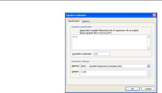
To estimate a quantile regression specification in EViews you may select Object/New Object.../Equation or Quick/Estimate Equation… from the main menu, or simply type the keyword equation in the command window. From the main estimation dialog you should select QREG - Quantile Regression (including LAD). Alternately, you may type qreg in the command window.

Estimating Quantile Regression in EViews—333

Quantile Regression Options

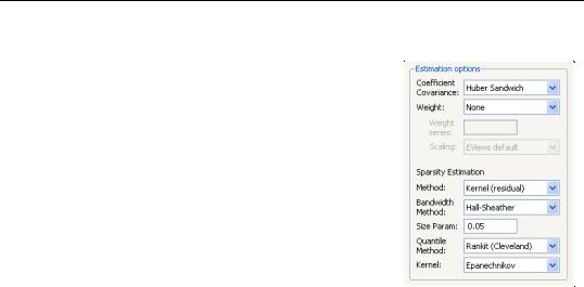
The combo box labeled Coefficient Covariance is where you will choose your method of computing covariances: computing Ordinary (IID) covariances, using a Huber Sandwich method, or using Bootstrap resampling. By default, EViews uses the Huber Sandwich calculations which are valid under independent but non-identical sampling.

Just below the combo box is an section Weight, where you may define observations weights. The data will be transformed prior to estimation using this specification.

(See “Weighted Least Squares” on page 36 for a discussion of the settings).

The remaining settings in this section control the estima-

tion of the scalar sparsity value. Different options are available for different Coefficient Covariance settings. For ordinary or bootstrap covariances you may choose either Siddiqui (mean fitted), Kernel (residual), or Siddiqui (residual) as your sparsity estimation method, while if the covariance method is set to Huber Sandwich, only the Siddiqui (mean fitted) and Kernel (residual) methods are available.

There are additional options for the bandwidth method (and associated size parameter if relevant), the method for computing empirical quantiles (used to estimate the sparsity or the kernel bandwidth), and the choice of kernel function. Most of these settings should be selfexplanatory; if necessary, see the discussion in “Sparsity Estimation,” beginning on

page 344 for details.

It is worth mentioning that the sparsity estimation options are always relevant, since EViews always computes and reports a scalar sparsity estimate, even if it is not used in computing the covariance matrix. In particular, a sparsity value is estimated even when you compute the asymptotic covariance using a Huber Sandwich method. The sparsity estimate will be used in non-robust quasi-likelihood ratio tests statistics as necessary.

Iteration Control

The iteration control section offers the standard edit field for changing the maximum number of iterations, a combo box for specifying starting values, and a check box for displaying the estimation settings in the output. Note that the default starting value for quantile regression is 0, but you may choose a fraction of the OLS estimates, or provide a set of user specified values.

Estimating Quantile Regression in EViews—335

Dependent Variable: Y

Method: Quantile Regression (Median)

Date: 08/12/09 Time: 11:46

Sample: 1 235

Included observations: 235

Huber Sandwich Standard Errors & Covariance

Sparsity method: Kernel (Epanechnikov) using residuals

Bandwidth method: Hall-Sheather, bw=0.15744

Estimation successfully identifies unique optimal solution

The top portion of the output displays the estimation settings. Here we see that our estimates use the Huber sandwich method for computing the covariance matrix, with individual sparsity estimates obtained using kernel methods. The bandwidth uses the Hall and Sheather formula, yielding a value of 0.15744.

Below the header information are the coefficients, along with standard errors, t-statistics and associated p-values. We see that both coefficients are statistically significantly different from zero and conventional levels.

The bottom portion of the output reports the Koenker and Machado (1999) goodness-of-fit measure (pseudo R-squared), and adjusted version of the statistic, as well as the scalar estimate of the sparsity using the kernel method. Note that this scalar estimate is not used in the computation of the standard errors in this case since we are employing the Huber sandwich method.

Also reported are the minimized value of the objective function (“Objective”), the minimized constant-only version of the objective (“Objective (const. only)”), the constant-only coefficient estimate (“Quantile dependent var”), and the corresponding Ln(t) form of the Quasi-LR statistic and associated probability for the difference between the two specifications (Koenker and Machado, 1999). Note that despite the fact that the coefficient covariances are computed using the robust Huber Sandwich, the QLR statistic assumes i.i.d. errors and uses the estimated value of the sparsity.

The reported S.E. of the regression is based on the usual d.f. adjusted sample variance of the residuals. This measure of scale is used in forming standardized residuals and forecast standard errors. It is replaced by the Koenker and Machado (1999) scale estimator in the compu-