

|
|
Working with Equations—17 |
|
|
|
|
|
|
|
|
|
|
@stderrs(i) |
standard error for coefficient i |
|
|
@tstats(i) |
t-statistic value for coefficient i |
|
|
|
|
|
|
c(i) |
i-th element of default coefficient vector for equation (if |
|
|
|
applicable) |
|
|
|
|
|
Selected Keywords that Return Vector or Matrix Objects |
|||
|
|
|
|
|
@coefcov |
matrix containing the coefficient covariance matrix |
|
|
|
|
|
|
@coefs |
vector of coefficient values |
|
|
|
|
|
|
@stderrs |
vector of standard errors for the coefficients |
|
|
|
|
|
|
@tstats |
vector of t-statistic values for coefficients |
|
|
|
|
|
Selected Keywords that Return Strings |
|||
|
|
|
|
|
@command |
full command line form of the estimation command |
|
|
|
|
|
|
@smpl |
description of the sample used for estimation |
|
|
|
|
|
|
@updatetime |
string representation of the time and date at which the |
|
|
|
equation was estimated |
|
|
|
|
|
See also “Equation” (p. 31) in the Object Reference for a complete list.
Functions that return a vector or matrix object should be assigned to the corresponding object type. For example, you should assign the results from @tstats to a vector:
vector tstats = eq1.@tstats
and the covariance matrix to a matrix:
matrix mycov = eq1.@cov
You can also access individual elements of these statistics:
scalar pvalue = 1-@cnorm(@abs(eq1.@tstats(4))) scalar var1 = eq1.@covariance(1,1)
For documentation on using vectors and matrices in EViews, see Chapter 8. “Matrix Language,” on page 159 of the Command and Programming Reference.
Working with Equations
Views of an Equation
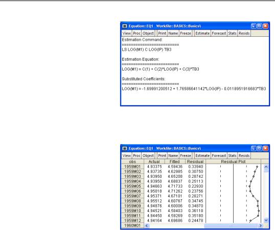
•Representations. Displays the equation in three forms: EViews command form, as an algebraic equation with symbolic coefficients, and as an equation with the estimated values of the coefficients.
18—Chapter 18. Basic Regression Analysis
You can cut-and-paste from the representations view into any application that supports the Windows clipboard.
•Estimation Output. Displays the equation output results described above.
•Actual, Fitted, Residual. These views display the actual and fitted values of
the dependent variable and the residuals from the regression in tabular and graphical form. Actual, Fitted, Residual Table displays these values in table form.
Note that the actual value is always the sum of the fitted value and the residual. Actual, Fitted, Residual Graph displays a standard EViews graph of the actual values, fitted values, and residuals.
Residual Graph plots only the residuals, while the
Standardized Residual Graph plots the residuals
divided by the estimated residual standard deviation.
•ARMA structure.... Provides views which describe the estimated ARMA structure of your residuals. Details on these views are provided in “ARMA Structure” on
page 104.
•Gradients and Derivatives. Provides views which describe the gradients of the objective function and the information about the computation of any derivatives of the regression function. Details on these views are provided in Appendix C. “Gradients and Derivatives,” on page 763.
•Covariance Matrix. Displays the covariance matrix of the coefficient estimates as a spreadsheet view. To save this covariance matrix as a matrix object, use the @cov function.
Working with Equations—19
•Coefficient Diagnostics, Residual Diagnostics, and Stability Diagnostics. These are views for specification and diagnostic tests and are described in detail in Chapter 23. “Specification and Diagnostic Tests,” beginning on page 139.
Procedures of an Equation
•Specify/Estimate…. Brings up the Equation Specification dialog box so that you can modify your specification. You can edit the equation specification, or change the estimation method or estimation sample.
•Forecast…. Forecasts or fits values using the estimated equation. Forecasting using equations is discussed in Chapter 22. “Forecasting from an Equation,” on page 111.
•Make Residual Series…. Saves the residuals from the regression as a series in the workfile. Depending on the estimation method, you may choose from three types of residuals: ordinary, standardized, and generalized. For ordinary least squares, only the ordinary residuals may be saved.
•Make Regressor Group. Creates an untitled group comprised of all the variables used in the equation (with the exception of the constant).
•Make Gradient Group. Creates a group containing the gradients of the objective function with respect to the coefficients of the model.
•Make Derivative Group. Creates a group containing the derivatives of the regression function with respect to the coefficients in the regression function.
•Make Model. Creates an untitled model containing a link to the estimated equation if a named equation or the substituted coefficients representation of an untitled equation. This model can be solved in the usual manner. See Chapter 34. “Models,” on page 511 for information on how to use models for forecasting and simulations.
•Update Coefs from Equation. Places the estimated coefficients of the equation in the coefficient vector. You can use this procedure to initialize starting values for various estimation procedures.
Residuals from an Equation
The residuals from the default equation are stored in a series object called RESID. RESID may be used directly as if it were a regular series, except in estimation.
RESID will be overwritten whenever you estimate an equation and will contain the residuals from the latest estimated equation. To save the residuals from a particular equation for later analysis, you should save them in a different series so they are not overwritten by the next estimation command. For example, you can copy the residuals into a regular EViews series called RES1 using the command:
series res1 = resid

20—Chapter 18. Basic Regression Analysis
There is an even better approach to saving the residuals. Even if you have already overwritten the RESID series, you can always create the desired series using EViews’ built-in procedures if you still have the equation object. If your equation is named EQ1, open the equation window and select Proc/Make Residual Series..., or enter:
eq1.makeresid res1
to create the desired series.
Storing and Retrieving an Equation
As with other objects, equations may be stored to disk in data bank or database files. You can also fetch equations from these files.
Equations may also be copied-and-pasted to, or from, workfiles or databases.
EViews even allows you to access equations directly from your databases or another workfile. You can estimate an equation, store it in a database, and then use it to forecast in several workfiles.
See Chapter 4. “Object Basics,” beginning on page 67 and Chapter 10. “EViews Databases,” beginning on page 267, both in User’s Guide I, for additional information about objects, databases, and object containers.
Using Estimated Coefficients
The coefficients of an equation are listed in the representations view. By default, EViews will use the C coefficient vector when you specify an equation, but you may explicitly use other coefficient vectors in defining your equation.
These stored coefficients may be used as scalars in generating data. While there are easier ways of generating fitted values (see “Forecasting from an Equation” on page 111), for purposes of illustration, note that we can use the coefficients to form the fitted values from an equation. The command:
series cshat = eq1.c(1) + eq1.c(2)*gdp
forms the fitted value of CS, CSHAT, from the OLS regression coefficients and the independent variables from the equation object EQ1.
Note that while EViews will accept a series generating equation which does not explicitly refer to a named equation:
series cshat = c(1) + c(2)*gdp
and will use the existing values in the C coefficient vector, we strongly recommend that you always use named equations to identify the appropriate coefficients. In general, C will contain the correct coefficient values only immediately following estimation or a coefficient