Working with a GLM Equation—315
Dependent Variable: PRATE
Method: Generalized Linear Model (Quadratic Hill Climbing) Date: 08/12/09 Time: 11:28
Sample: 1 4735 IF MRATE <=1 Included observations: 3784
Family: Binomial Proportion (trials = 1) Link: Logit
Dispersion fixed at 1
Coefficient covariance computed using the Huber-White method with observed Hessian
Convergence achieved after 8 iterations
Variable |
Coefficient |
Std. Error |
z-Statistic |
Prob. |
|
|
|
|
|
|
|
|
|
|
MRATE |
1.390080 |
0.107792 |
12.89596 |
0.0000 |
LOG(TOTEMP) |
-1.001875 |
0.110524 |
-9.064762 |
0.0000 |
LOG(TOTEMP)^2 |
0.052187 |
0.007134 |
7.315686 |
0.0000 |
AGE |
0.050113 |
0.008852 |
5.661090 |
0.0000 |
AGE^2 |
-0.000515 |
0.000212 |
-2.432325 |
0.0150 |
SOLE |
0.007947 |
0.050242 |
0.158171 |
0.8743 |
C |
5.058001 |
0.421199 |
12.00858 |
0.0000 |
|
|
|
|
|
|
|
|
Mean dependent var |
0.847769 |
S.D. dependent var |
0.169961 |
Sum squared resid |
92.69516 |
Log likelihood |
|
-1179.279 |
Akaike info criterion |
0.626997 |
Schwarz criterion |
0.638538 |
Hannan-Quinn criter. |
0.631100 |
Deviance |
|
765.0353 |
Deviance statistic |
0.202551 |
Restr. deviance |
895.5505 |
LR statistic |
130.5153 |
Prob(LR statistic) |
0.000000 |
Pearson SSR |
724.4200 |
Pearson statistic |
0.191798 |
Dispersion |
1.000000 |
|
|
|
|
|
|
|
|
|
|
|
|
|
EViews reports the new method of computing the coefficient covariance in the header. The coefficient estimates are unchanged, since the alternative computation of the coefficient covariance is a post-estimation procedure, and the new standard estimates correspond the second set of standard errors in Papke and Wooldridge (Table II, column 2). Notably, the use of an alternative estimator for the coefficient covariance has little substantive effect on the results.
Working with a GLM Equation
EViews offers various views and procedures for a estimated GLM equation. Some, like the Gradient Summary or the coefficient Covariance Matrix view are self-explanatory. In this section, we offer relevant comment on the remaining views.
Residuals
The main equation output offers summary statistics for the sum-of-squared response residuals (“Sum squared resid”), and the sum-of-squared Pearson residuals (“Pearson SSR”).
316—Chapter 27. Generalized Linear Models
The Actual, Fitted, Residual views and Residual Diagnostics allow you to examine properties of your residuals. The Actual, Fitted, Residual Table and Graph, show the fit of the unweighted data. As the name suggests, the Standardized Residual Graph displays the standardized (scaled Pearson) residuals.
The Residual Diagnostics show Histograms of the standardized residuals and Correlograms of the standardized residuals and the squared standardized residuals.
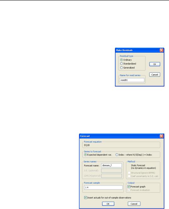
The Make Residuals proc allows you to save the Ordinary (response), Standardized (scaled Pearson), or Generalized (score) residuals into the workfile. The latter may be useful for constructing test statistics (note, however, that in some cases, it may be more useful to compute the gradients of the model directly using Proc/Make Gradient Group).
Given standardized residuals SRES for equation EQ1, the unscaled Pearson residuals may be obtained using the command
series pearson = sres * @sqrt(eq1.@dispersion)
Forecasting
EViews offers built-in tools for producing in and out-of-sample forecasts (fits) from your GLM estimated equation. Simply click on the Forecast button on your estimated equation to bring up the forecast dialog, then enter the desired settings.
You should first use the radio buttons to specify whether you wish to forecast the expected dependent variable mi or the linear index hi .
Next, enter the name of the series to hold the forecast output, and set the forecast sample.
Lastly, specify whether you wish to produce a forecast graph and whether you wish to fill non-fore- cast values in the workfile with actual values or to fill them with NAs. For most cross-section applications, we recommend that you uncheck this box.
Click on OK to produce the forecast.
Working with a GLM Equation—317
Note that while EViews does not presently offer a menu item for saving the fitted GLM variances or scaled variances, you can easily obtain results by saving the ordinary and standardized residuals and taking ratios (“Residuals” on page 328). If ORESID are the ordinary and SRESID are the standardized residuals for equation EQ1, then the commands
series glmsvar = (oresid / sresid)^2
series glmvar = glmvar * eq1.@dispersion
produce the scaled variance and unscaled variances, respectively.
Lastly, you should use Proc/Make Model to create a model object for more complicated simulation from your GLM equation.
Testing
You may perform Wald tests of coefficient restrictions. Simply select View/Coefficient Diagnostics/Wald - Coefficient Restrictions, then enter your restrictions in the edit field. For the Papke-Wooldridge example above with Huber-White robust covariances, we may use a Wald test to evaluate the joint significance of AGE^2 and SOLE by entering the restriction “C(5)=C(6)=0” and clicking on OK to perform the test.
Wald Test:
Equation: EQ2_QMLE_R
Null Hypothesis: C(5)=C(6)=0
Test Statistic |
Value |
df |
Probability |
|
|
|
|
|
|
|
|
F-statistic |
2.970226 |
(2, 3777) |
0.0514 |
Chi-square |
5.940451 |
2 |
0.0513 |
|
|
|
|
|
|
Null Hypothesis Summary: |
|
|
|
|
|
|
|
|
|
Normalized Restriction (= 0) |
Value |
Std. Err. |
|
|
|
|
|
|
|
|
C(5) |
|
-0.000515 |
0.000212 |
C(6) |
|
0.007947 |
0.050242 |
|
|
|
|
|
|
|
|
Restrictions are linear in coefficients.
The test results show joint-significance at just above the 5% level. The Confidence Intervals and Confidence Ellipses... views will also employ the robust covariance matrix estimates.
The Omitted Variables... and Redundant Variables... views and the Ramsey RESET Test... views are likelihood ratio based tests. Note that the RESET test is a special case of an omitted variables test where the omitted variables are powers of the fitted values from the original equation.
318—Chapter 27. Generalized Linear Models
We illustrate these tests by performing the RESET test on the first Papke-Wooldridge QMLE equation with GLM covariances. Select View/Stability Diagnostics/Ramsey Reset Test...
and change the default to include 2 fitted terms in the test equation.
Ramsey RESET Test
Equation: EQ2_QMLE
Specification: PRATE MRATE LOG(TOTEMP) LOG(TOTEMP)^2 AGE
AGE^2 SOLE C
Omitted Variables: Powers of fitted values from 2 to 3
|
Value |
df |
Probability |
|
F-statistic |
0.311140 |
(2, 3775) |
0.7326 |
|
QLR* statistic |
0.622280 |
2 |
0.7326 |
|
|
|
|
|
|
|
|
|
|
|
F-test summary: |
|
|
Mean |
|
|
|
|
|
|
Sum of Sq. |
df |
Squares |
|
Test Deviance |
0.119389 |
2 |
0.059694 |
|
Restricted Deviance |
765.0353 |
3777 |
0.202551 |
|
Unrestricted Deviance |
764.9159 |
3775 |
0.202627 |
|
Dispersion SSR |
724.2589 |
3775 |
0.191857 |
|
|
|
|
|
|
|
|
|
|
|
QLR* test summary: |
|
|
|
|
|
Value |
df |
|
|
Restricted Deviance |
765.0353 |
3777 |
|
|
Unrestricted Deviance |
764.9159 |
3775 |
|
|
Dispersion |
0.191857 |
|
|
|
|
|
|
|
|
|
|
|
|
|
The top portion of the output shows the test settings, and the test summaries. The bottom portion of the output shows the estimated test equation. The results show little evidence of nonlinearity.
Notice that in contrast to LR tests in most other equation views, the likelihood ratio test statistics in GLM equations are obtained from analysis of the deviances or quasi-deviances.
Suppose D0 is the unscaled deviance under the null and D1 is the corresponding statistic |
under the alternative hypothesis. The usual asymptotic x2 |
likelihood ratio test statistic may |
be written in terms of the difference of deviances with common scaling, |
D0 – D1 |
~ x |
2 |
(27.4) |
------------------- |
r |
ˆ |
|
|
f |
|
|
|
ˆ |
|
|
r is the fixed number of restric- |
as N Æ •, where f is an estimate of the dispersion and |
tions imposed by the null hypothesis. ˆ is either a specified fixed value or an estimate f
under the alternative hypothesis using the specified dispersion method. When D0 and D1 contain the quasi-deviances, the resulting statistic is the quasi-likelihood ratio (QLR) statistic (Wooldridge, 1997).
If f is estimated, we may also employ the F-statistic variant of the test statistic:
(D0 – D1) § r |
~ Fr, N – p |
(27.5) |
-------------------------------ˆ |
f |
|
|