Chapter 27. Generalized Linear Models
Nelder and McCullagh (1972) describe a class of Generalized Linear Models (GLMs) that extends linear regression to permit non-normal stochastic and non-linear systematic components. GLMs encompass a broad and empirically useful range of specifications that includes linear regression, logistic and probit analysis, and Poisson models.
GLMs offer a common framework in which we may place all of these specification, facilitating development of broadly applicable tools for estimation and inference. In addition, the GLM framework encourages the relaxation of distributional assumptions associated with these models, motivating development of robust quasi-maximum likelihood (QML) estimators and robust covariance estimators for use in these settings.
The following discussion offers an overview of GLMs and describes the basics of estimating and working with GLMs in EViews. Those wishing additional background and technical information are encouraged to consult one of the many excellent summaries that are available (McCullagh and Nelder 1989, Hardin and Hilbe 2007, Agresti 1990).
Overview
Suppose we have i = 1, º, N independent response variables Yi , each of whose conditional mean depends on k -vectors of explanatory variables Xi and unknown coefficients b . We may decompose Yi into a systematic mean component, mi , and a stochastic component ei
The conventional linear regression model assumes that the mi is a linear predictor formed from the explanatory variables and coefficients, mi = Xi¢b , and that ei is normally distributed with zero mean and constant variance Vi = j2 .
The GLM framework of Nelder and McCullagh (1972) generalizes linear regression by allowing the mean component mi to depend on a linear predictor through a nonlinear function, and the distribution of the stochastic component ei be any member of the linear exponential family. Specifically, a GLM specification consists of:
• A linear predictor or index hi = Xi¢b + oi where oi is an optional offset term.
•A distribution for Yi belonging to the linear exponential family.
•A smooth, invertible link function, g(mi) = hi , relating the mean mi and the linear predictor hi .
A wide range of familiar models may be cast in the form of a GLM by choosing an appropriate distribution and link function. For example:
302—Chapter 27. Generalized Linear Models
Model |
Family |
Link |
|
|
|
Linear Regression |
Normal |
Identity: g(m) = m |
|
|
|
Exponential Regression |
Normal |
Log: g(m) = log(m) |
|
|
|
Logistic Regression |
Binomial |
Logit: g(m) = log(m § (1 – m)) |
|
|
|
Probit Regression |
Binomial |
Probit: g(m) = F–1(m) |
|
|
|
Poisson Count |
Poisson |
Log: g(m) = log(m) |
|
|
|
For a detailed description of these and other familiar specifications, see McCullagh and Nelder (1981) and Hardin and Hilbe (2007). It is worth noting that the GLM framework is able to nest models for continuous (normal), proportion (logistic and probit), and discrete count (Poisson) data.
Taken together, the GLM assumptions imply that the first two moments of Yi may be written as functions of the linear predictor:
mi = g–1(hi )
(27.2)
Vi = (f § wi )Vm (g–1(hi))
where Vm (m) is a distribution-specific variance function describing the mean-variance relationship, the dispersion constant f > 0 is a possibly known scale factor, and wi > 0 is a known prior weight that corrects for unequal scaling between observations.
Crucially, the properties of the GLM maximum likelihood estimator depend only on these two moments. Thus, a GLM specification is principally a vehicle for specifying a mean and variance, where the mean is determined by the link assumption, and the mean-variance relationship is governed by the distributional assumption. In this respect, the distributional assumption of the standard GLM is overly restrictive.
Accordingly, Wedderburn (1974) shows that one need only specify a mean and variance specification as in Equation (27.2) to define a quasi-likelihood that may be used for coefficient and covariance estimation. Not surprisingly, for variance functions derived from exponential family distributions, the likelihood and quasi-likelihood functions coincide. McCullagh (1983) offers a full set of distributional results for the quasi-maximum likelihood (QML) estimator that mirror those for ordinary maximum likelihood.
QML estimators are an important tool for the analysis of GLM and related models. In particular, these estimators permit us to estimate GLM-like models involving mean-variance specifications that extend beyond those for known exponential family distributions, and to estimate models where the mean-variance specification is of exponential family form, but
How to Estimate a GLM in EViews—303
the observed data do not satisfy the distributional requirements (Agresti 1990, 13.2.3 offers a nice non-technical overview of QML).
Alternately, Gourioux, Monfort, and Trognon (1984) show that consistency of the GLM maximum likelihood estimator requires only correct specification of the conditional mean. Misspecification of the variance relationship does, however, lead to invalid inference, though this may be corrected using robust coefficient covariance estimation. In contrast to the QML results, the robust covariance correction does not require correction specification of a GLM conditional variance.
How to Estimate a GLM in EViews
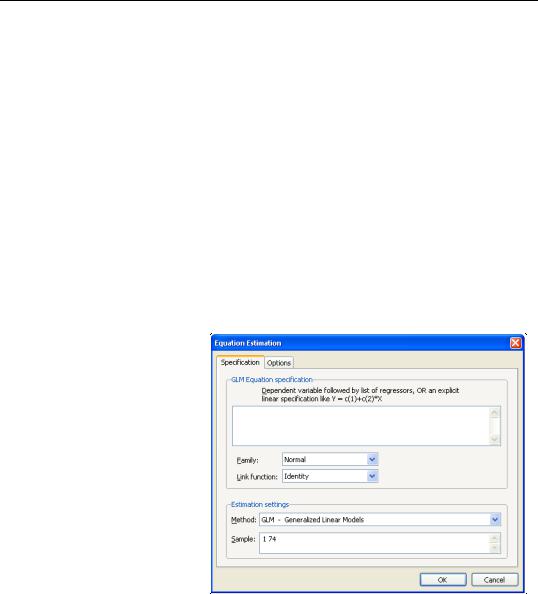
To estimate a GLM model in EViews you must first create an equation object. You may select Object/New Object.../Equation or Quick/Estimate Equation… from the main menu, or enter the keyword equation in the command window. Next select GLM - Generalized Linear Model in the Method combo box. Alternately, entering the keyword glm in the command window will both create the object and automatically set the estimation method. The dialog will change to show settings appropriate for specifying a GLM.
Specification
The main page of the dialog is used to describe the basic GLM specification.
We will focus attention on the GLM Equation specification section since the
Estimation settings section in the bottom of the dialog is should be self-explana- tory.
Dependent Variable and
Linear Predictor
In the main edit field you should specify your depen-
dent variable and the linear predictor.
There are two ways in which you may enter this information. The easiest method is to list the dependent response variable followed by all of the regressors that enter into the predictor. PDL specifications are permitted in this list, but ARMA terms are not. If you wish to include an offset in your predictor, it should be entered on the Options page (see “Specification Options” on page 305).
304—Chapter 27. Generalized Linear Models
Alternately, you may enter an explicit linear specification like “Y=C(1)+C(2)*X”. The response variable will be taken to be the variable on the left-hand side of the equality (“Y”) and the linear predictor will be taken from the right-hand side of the expression (“C(1)+C(2)*X”). Offsets may be entered directly in the expression or they may be entered on the Options page. Note that this specification should not be taken as a literal description of the mean equation; it is merely a convenient syntax for specifying both the response and the linear predictor.
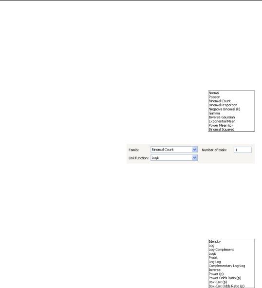
Family
Next, you should use the Family combo to specify your distribution. The default family is the Normal distribution, but you are free to choose from the list of linear exponential family and quasi-likelihood distributions. Note that the last three entries (Exponential Mean, Power Mean (p), Binomial Squared) are for quasi-likelihood specifications not associated with exponential families.
If the selected distribution requires specification of an ancillary parameter, you will be prompted to provide the values. For example, the Bino-
mial Count and Binomial Proportion distributions both require specification of the number of trials ni , while the Negative Binomial requires specification of the excess-variance parameter ki .
For descriptions of the various exponential and quasi-likelihood families, see “Distribution,” beginning on page 319.
Link
Lastly, you should use the Link combo to specify a link function.
EViews will initialize the Link setting to the default for to the selected family. In general, the canonical link is used as the default link, however, the Log link is used as the default for the Negative Binomial family. The Exponential Mean, Power Mean (p), and Binomial Squared quasi-likelihood families will default to use the Identity, Log, and Logit links, respectively.
If the link that you select requires specification of parameter values, you will be prompted to enter the values.
For detailed descriptions of the link functions, see “Link,” beginning on page 321.
How to Estimate a GLM in EViews—305
Options
Click on the Options tab to display additional settings for the GLM specification. You may use this page to augment the equation specification, to choose a dispersion estimator, to specify the estimation algorithm and associated settings, or to define a coefficient covariance estimator.
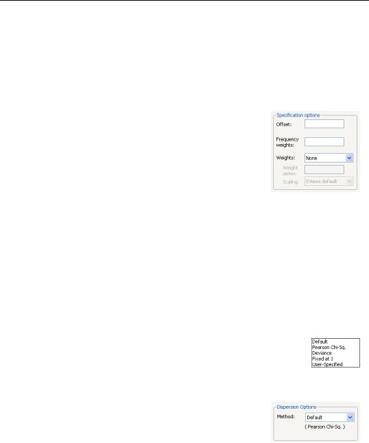
Specification Options
The Specification Options section of the Options tab allows you to augment the GLM specification.
To include an offset in your linear predictor, simply enter a series name or expression in the Offset edit field.
The Frequency weights edit field should be used to specify replicates for each observation in the workfile. In practical terms, the frequency weights act as a form of variance weight-
ing and inflate the number of “observations” associated with the data records.
You may also specify prior variance weights in the using the Weights combo and associated edit fields. To specify your weights, simply select a description for the form of the weighting series (Inverse std. dev., Inverse variance, Std. deviation, Variance), then enter the corresponding weight series name or expression. EViews will translate the values in the weighting series into the appropriate values for wi . For example, to specify wi directly, you should select Inverse variance then enter the series or expression containing the wi values. If you instead choose Variance, EViews will set wi to the inverse of the values in the weight series. “Weighted Least Squares” on page 36 for additional discussion.
Dispersion Options
The Method combo may be used to select the dispersion computation method. You will always be given the opportunity to choose between the
Default setting or Pearson Chi-Sq., Fixed at 1, and User-Specified. Additionally, if the specified distribution is in the linear exponential family, you may choose to use the Deviance statistic.
The Default entry instructs EViews to use the default method for computing the dispersion, which will depend on the specified family. For families with a free dispersion parameter, the default is to use the Pearson Chi-Sq. statistic, otherwise the default is Fixed at 1. The current default setting will be displayed directly below the combo.
306—Chapter 27. Generalized Linear Models
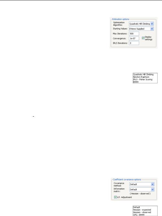
Estimation Options
The Estimation options section of the page lets you specify the algorithm, starting values, and other estimation settings.
You may use the Optimization Algorithm combo used to choose your estimation method. The default is to use Quadratic Hill Climbing, a Newton-Raphson variant, or you may select Newton-Raphson, IRLS - Fisher Scoring,
or BHHH. The first two methods use the observed information matrix to weight the gradients in coefficient updates, while the latter two methods weight using the expected information and outer-product of the gradients, respectively.
Note that while the algorithm choice will generally not matter for the coefficient estimates, it does have implications for the default computation of standard errors since EViews will, by default, use the implied
estimator of the information matrix in computing the coefficient covariance (see “Coefficient Covariance Options” on page 306 for details).
By default, the Starting Values combo is set to EViews Supplied. The EViews default starting values for b are obtained using the suggestion of McCullagh and Nelder to initialize the IRLS algorithm at mˆ i = (niyi + 0.5) § (ni + 1) for the binomial proportion family, and
mˆ i = (yi + y) § 2 otherwise, then running a single IRLS coefficient update to obtain the initial b . Alternately, you may specify starting values that are a fraction of the default values, or you may instruct EViews to use your own values.
You may use the IRLS iterations edit field to instruct EViews to perform a fixed number of additional IRLS updates to refine coefficient values prior to starting the specified estimation algorithm.
The Max Iterations and Convergence edit fields are self-explanatory. Selecting the Display settings checkbox instructs EViews to show detailed information on tolerances and initial values in the equation output.
Coefficient Covariance Options
The Covariance method combo specifies the estimator for the coefficient covariance matrix. You may choose between the Default method, which uses the inverse of the estimated information matrix, or you may elect to use Huber/White sandwich estimator.
The Information matrix combo allows you to specify the method for estimating the information matrix. For covariances computed using the inverse information matrix, you may choose between the Default set-