Count Models

Count Models—289

Negative Binomial (ML)

One common alternative to the Poisson model is to estimate the parameters of the model using maximum likelihood of a negative binomial specification. The log likelihood for the negative binomial distribution is given by:

i = 1

+ logG(yi + 1 § h2 )–log(yi!)–logG(1 § h2)

where h2 is a variance parameter to be jointly estimated with the conditional mean parameters b . EViews estimates the log of h2 , and labels this parameter as the “SHAPE” parameter in the output. Standard errors are computed using the inverse of the information matrix.

The negative binomial distribution is often used when there is overdispersion in the data, so that v(xi, b) > m(xi, b), since the following moment conditions hold:

E(yi xi, b) = m(xi, b)

(26.45)

var(yi xi, b) = m(xi, b)(1 + h2m(xi, b))

h2 is therefore a measure of the extent to which the conditional variance exceeds the conditional mean.

Consistency and efficiency of the negative binomial ML requires that the conditional distribution of y be negative binomial.

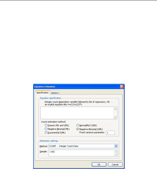
Quasi-maximum Likelihood (QML)

We can perform maximum likelihood estimation under a number of alternative distributional assumptions. These quasi-maximum likelihood (QML) estimators are robust in the sense that they produce consistent estimates of the parameters of a correctly specified conditional mean, even if the distribution is incorrectly specified.

This robustness result is exactly analogous to the situation in ordinary regression, where the normal ML estimator (least squares) is consistent, even if the underlying error distribution is not normally distributed. In ordinary least squares, all that is required for consistency is a correct specification of the conditional mean m(xi, b) = xi¢b . For QML count models, all that is required for consistency is a correct specification of the conditional mean m(xi, b).

The estimated standard errors computed using the inverse of the information matrix will not be consistent unless the conditional distribution of y is correctly specified. However, it is possible to estimate the standard errors in a robust fashion so that we can conduct valid inference, even if the distribution is incorrectly specified.

Count Models—291

Negative Binomial

If we maximize the negative binomial log likelihood, given above, for fixed h2 , we obtain the QMLE of the conditional mean parameters b . This QML estimator is consistent even if the conditional distribution of y is not negative binomial, provided that mi is correctly specified.

EViews sets h2 = 1 by default, which is a special case known as the geometric distribution. You may specify any other (positive) value by changing the number in the Fixed variance parameter field box. For the negative binomial QMLE, EViews by default reports the robust QMLE standard errors.

Views of Count Models

EViews provides a full complement of views of count models. You can examine the estimation output, compute frequencies for the dependent variable, view the covariance matrix, or perform coefficient tests. Additionally, you can select View/Actual, Fitted, Residual… and

can examine the correlogram and histogram of these residuals. For the most part, all of these views are self-explanatory.

Note, however, that the LR test statistics presented in the summary statistics at the bottom of the equation output, or as computed under the View/Coefficient Diagnostics/Redundant Variables - Likelihood Ratio… have a known asymptotic distribution only if the conditional distribution is correctly specified. Under the weaker GLM assumption that the true variance is proportional to the nominal variance, we can form a quasi-likelihood ratio, QLR = LR § jˆ 2 , where jˆ 2 is the estimated proportional variance factor. This QLR statistic has an asymptotic x2 distribution under the assumption that the mean is correctly specified and that the variances follow the GLM structure. EViews does not compute the QLR statistic, but it can be estimated by computing an estimate of jˆ 2 based upon the standardized residuals. We provide an example of the use of the QLR test statistic below.

If the GLM assumption does not hold, then there is no usable QLR test statistic with a known distribution; see Wooldridge (1997).

Procedures for Count Models

Most of the procedures are self-explanatory. Some details are required for the forecasting and residual creation procedures.

•Make Residual Series… provides the following three types of residuals for count models:

Count Models—293

Dependent Variable: NUMB

Method: ML/QML - Poisson Count (Quadratic hill climbing)

Date: 08/12/09 Time: 09:55

Sample: 1 103

Included observations: 103

Convergence achieved after 4 iterations

Covariance matrix computed using second derivatives

Cameron and Trivedi (1990) propose a regression based test of the Poisson restriction

v(xi, b) = m(xi, b). To carry out the test, first estimate the Poisson model and obtain the fitted values of the dependent variable. Click Forecast and provide a name for the forecasted dependent variable, say NUMB_F. The test is based on an auxiliary regression of e2oi – yi on yˆ 2i and testing the significance of the regression coefficient. For this example, the test regression can be estimated by the command:

equation testeq.ls (numb-numb_f)^2-numb numb_f^2

yielding the following results:

Dependent Variable: (NUMB-NUMB_F)^2-NUMB

Method: Least Squares

Date: 08/12/09 Time: 09:57

Sample: 1 103

Included observations: 103

Count Models—295

Dependent Variable: NUMB

Method: QML - Negative Binomial Count (Quadratic hill climbing)

Date: 08/12/09 Time: 10:55

Sample: 1 103

Included observations: 103

QML parameter used in estimation: 0.22124

Convergence achieved after 4 iterations

GLM Robust Standard Errors & Covariance

Variance factor estimate = 0.989996509662

Covariance matrix computed using second derivatives

The negative binomial QML should be consistent, and under the GLM assumption, the standard errors should be consistently estimated. It is worth noting that the coefficient on FEB, which was strongly statistically significant in the Poisson specification, is no longer significantly different from zero at conventional significance levels.

Quasi-likelihood Ratio Statistic

As described by Wooldridge (1997), specification testing using likelihood ratio statistics requires some care when based upon QML models. We illustrate here the differences between a standard LR test for significant coefficients and the corresponding QLR statistic.

From the results above, we know that the overall likelihood ratio statistic for the Poisson model is 16.85, with a corresponding p-value of 0.0002. This statistic is valid under the assumption that m(xi, b) is specified correctly and that the mean-variance equality holds.

We can decisively reject the latter hypothesis, suggesting that we should derive the QML estimator with consistently estimated covariance matrix under the GLM variance assumption. While EViews currently does not automatically adjust the LR statistic to reflect the QML assumption, it is easy enough to compute the adjustment by hand. Following Wooldridge, we construct the QLR statistic by dividing the original LR statistic by the estimated GLM variance factor. (Alternately, you may use the GLM estimators for count models described in Chapter 27. “Generalized Linear Models,” on page 301, which do compute the QLR statistics automatically.)