To create a series containing the generalized residuals, select View/Make Residual Series…, enter a name or accept the default name, and click OK. The generalized residuals for an ordered model are given by:
In some settings, the dependent variable is only partially observed. For example, in survey data, data on incomes above a specified level are often top-coded to protect confidentiality. Similarly desired consumption on durable goods may be censored at a small positive or zero value. EViews provides tools to perform maximum likelihood estimation of these models and to use the results for further analysis.
Background
Consider the following latent variable regression model:
yi = xi¢b + jei ,
(26.24)
where j is a scale parameter. The scale parameter j is identified in censored and truncated regression models, and will be estimated along with the b .
In the canonical censored regression model, known as the tobit (when there are normally distributed errors), the observed data y are given by:
yi £ 0
yi
=
0
if
yi
(26.25)
if
yi > 0
In other words, all negative values of yi are coded as 0. We say that these data are left censored at 0. Note that this situation differs from a truncated regression model where negative values of yi are dropped from the sample. More generally, EViews allows for both left and right censoring at arbitrary limit points so that:
ci
yi £ ci
if
yi
=
y
if
c
< y
£ c
i
i
(26.26)
i
i
ci
if
ci < yi
274—Chapter 26. Discrete and Limited Dependent Variable Models
where ci , ci are fixed numbers representing the censoring points. If there is no left censoring, then we can set ci = –•. If there is no right censoring, then ci = •. The canonical tobit model is a special case with ci = 0 and ci = •.
The parameters b , j are estimated by maximizing the log likelihood function:
N
l(b, j) =
 logf((yi – xi¢b) § j) 1(ci < yi < ci)
(26.27)
i
= 1
N
+
 log(F((ci – xi¢b) § j)) 1(yi = ci )
N
i = 1
+ Â log(1 – F((ci – xi¢b) § j)) 1(yi = ci )
i = 1
where f , F are the density and cumulative distribution functions of e , respectively.
Estimating Censored Models in EViews
Suppose that we wish to estimate the model:
HRSi = b1 + b2AGEi + b3EDUi + b4KID1i + ei ,
(26.28)
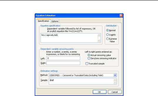
where hours worked (HRS) is left censored at zero. To estimate this model, select Quick/ Estimate Equation… from the main menu. Then from the Equation Estimation dialog, select the CENSORED - Censored or Truncated Data (including Tobit) estimation method. Alternately, enter the keyword censored in the command line and press ENTER. The dialog will change to provide a number of different input options.
Specifying the Regression Equation
In the Equation specification field, enter the name of the censored dependent variable followed by a list of regressors or an explicit expression for the equation. In our example, you will enter:
hrs c age edu kid1
Censored Regression Models—275
Next, select one of the three distributions for the error term. EViews allows you three possible choices for the distribution of e :
Standard normal
E(e)
= 0 , var(e) = 1
Logistic
E(e)
= 0 , var(e) = p2 § 3
Extreme value (Type I)
E(e) ª –0.5772(Euler’s constant),
var(e) = p2 § 6
Bear in mind that the extreme value distribution is asymmetric.
Specifying the Censoring Points
You must also provide information about the censoring points of the dependent variable. There are two cases to consider: (1) where the limit points are known for all individuals, and (2) where the censoring is by indicator and the limit points are known only for individuals with censored observations.
Limit Points Known
You should enter expressions for the left and right censoring points in the edit fields as required. Note that if you leave an edit field blank, EViews will assume that there is no censoring of observations of that type.
276—Chapter 26. Discrete and Limited Dependent Variable Models
For example, in the canonical tobit model the data are censored on the left at zero, and are uncensored on the right. This case may be specified as:
Left edit field: 0
Right edit field: [blank]
Similarly, top-coded censored data may be specified as,
Left edit field: [blank]
Right edit field: 20000
while the more general case of left and right censoring is given by: Left edit field: 10000
Right edit field: 20000
EViews also allows more general specifications where the censoring points are known to differ across observations. Simply enter the name of the series or auto-series containing the censoring points in the appropriate edit field. For example:
Left edit field: lowinc
Right edit field: vcens1+10
specifies a model with LOWINC censoring on the left-hand side, and right censoring at the value of VCENS1+10.
Limit Points Not Known
In some cases, the hypothetical censoring point is unknown for some individuals (ci and ci are not observed for all observations). This situation often occurs with data where censoring is indicated with a zero-one dummy variable, but no additional information is provided about potential censoring points.
EViews provides you an alternative method of describing data censoring that matches this format. Simply select the Field is zero/one indicator of censoring option in the estimation dialog, and enter the series expression for the censoring indicator(s) in the appropriate edit field(s). Observations with a censoring indicator of one are assumed to be censored while those with a value of zero are assumed to be actual responses.
For example, suppose that we have observations on the length of time that an individual has been unemployed (U), but that some of these observations represent ongoing unemployment at the time the sample is taken. These latter observations may be treated as right censored at the reported value. If the variable RCENS is a dummy variable representing censoring, you can click on the Field is zero/one indicator of censoring setting and enter:
Left edit field: [blank]
Right edit field: rcens
Censored Regression Models—277
in the edit fields. If the data are censored on both the left and the right, use separate binary indicators for each form of censoring:
Left edit field: lcens
Right edit field: rcens
where LCENS is also a binary indicator.
Once you have specified the model, click OK. EViews will estimate the parameters of the model using appropriate iterative techniques.
A Comparison of Censoring Methods
An alternative to specifying index censoring is to enter a very large positive or negative value for the censoring limit for non-censored observations. For example, you could enter “1e-100” and “1e100” as the censoring limits for an observation on a completed unemployment spell. In fact, any limit point that is “outside” the observed data will suffice.
While this latter approach will yield the same likelihood function and therefore the same parameter values and coefficient covariance matrix, there is a drawback to the artificial limit approach. The presence of a censoring value implies that it is possible to evaluate the conditional mean of the observed dependent variable, as well as the ordinary and standardized residuals. All of the calculations that use residuals will, however, be based upon the arbitrary artificial data and will be invalid.
If you specify your censoring by index, you are informing EViews that you do not have information about the censoring for those observations that are not censored. Similarly, if an observation is left censored, you may not have information about the right censoring limit. In these circumstances, you should specify your censoring by index so that EViews will prevent you from computing the conditional mean of the dependent variable and the associated residuals.
Interpreting the Output
If your model converges, EViews will display the estimation results in the equation window. The first part of the table presents the usual header information, including information about the assumed error distribution, estimation sample, estimation algorithms, and number of iterations required for convergence.
EViews also provides information about the specification for the censoring. If the estimated model is the canonical tobit with left-censoring at zero, EViews will label the method as a TOBIT. For all other censoring methods, EViews will display detailed information about form of the left and/or right censoring.
Here, we see an example of header output from a left censored model (our example below) where the censoring is specified by value:
278—Chapter 26. Discrete and Limited Dependent Variable Models
Dependent Variable: Y_PT
Method: ML - Censored Normal (TOBIT) (Quadratic hill climbing)
Date: 08/12/09 Time: 01:01
Sample: 1 601
Included observations: 601
Left censoring (value) at zero
Convergence achieved after 7 iterations
Covariance matrix computed using second derivatives
Below the header are the usual results for the coefficients, including the asymptotic standard errors, z-statistics, and significance levels. As in other limited dependent variable models, the estimated coefficients do not have a direct interpretation as the marginal effect of the associated regressor j for individual i , xij . In censored regression models, a change in xij has two effects: an effect on the mean of y , given that it is observed, and an effect on the probability of y being observed (see McDonald and Moffitt, 1980).
In addition to results for the regression coefficients, EViews reports an additional coefficient named SCALE, which is the estimated scale factor j . This scale factor may be used to esti-
mate the standard deviation of the residual, using the known variance of the assumed distribution. For example, if the estimated SCALE has a value of 0.4766 for a model with
extreme value errors, the implied standard error of the error term is
0.5977 = 0.466p § 6 .
Most of the other output is self-explanatory. As in the binary and ordered models above, EViews reports summary statistics for the dependent variable and likelihood based statistics. The regression statistics at the bottom of the table are computed in the usual fashion,
ˆ
=
yi – E(yi
ˆ
ˆ
y .
using the residuals ei
xi, b, j) from the observed
Views of Censored Equations
Most of the views that are available for a censored regression are familiar from other settings. The residuals used in the calculations are defined below.
The one new view is the Categorical Regressor Stats view, which presents means and standard deviations for the dependent and independent variables for the estimation sample. EViews provides statistics computed over the entire sample, as well as for the left censored, right censored and non-censored individuals.
Procedures for Censored Equations
EViews provides several procedures which provide access to information derived from your censored equation estimates.
Make Residual Series
Select Proc/Make Residual Series, and select from among the three types of residuals. The three types of residuals for censored models are defined as:
where f , F are the density and distribution functions, and where 1 is an indicator function which takes the value 1 if the condition in parentheses is true, and 0 if it is false. All of the above terms will be evaluated at the estimated b and j . See the discussion of forecasting for details on the computation of E(yi xi, b, j).
The generalized residuals may be used as the basis of a number of LM tests, including LM tests of normality (see Lancaster, Chesher and Irish (1985), Chesher and Irish (1987), and Gourioux, Monfort, Renault and Trognon (1987); Greene (2008), provides a brief discussion and additional references).
Forecasting
EViews provides you with the option of forecasting the expected dependent variable,
E(yi xi, b, j), or the expected latent variable, E(yi xi, b, j). Select Forecast from the equation toolbar to open the forecast dialog.
To forecast the expected latent variable, click on Index - Expected latent variable, and enter a name for the series to hold the output. The forecasts of the expected latent variable E(yi xi, b, j) may be derived from the latent model using the relationship:
ˆ
=
E(yi
ˆ ˆ
=
ˆ
ˆ
(26.29)
yi
xi, b, j)
xi¢b – jg .
where g is the Euler-Mascheroni constant (g ª 0.5772156649 ).
To forecast the expected observed dependent variable, you should select Expected dependent variable, and enter a series name. These forecasts are computed using the relationship:
ˆ
= E(yi
ˆ ˆ
yi
xi, b, j) =
+ E(yi
ci < yi < ci ;
+ ci Pr(yi = ci
ˆ
xi, b,
ci Pr(yi = ci
ˆ
ˆ
(26.30)
xi, b, j)
ˆ
ˆ ˆ
< ci
ˆ
xi, b, j) Pr(ci < yi
xi, b, j)
jˆ )
280—Chapter 26. Discrete and Limited Dependent Variable Models
Note that these forecasts always satisfy ci £ yˆ i £ ci . The probabilities associated with being in the various classifications are computed by evaluating the cumulative distribution function of the specified distribution. For example, the probability of being at the lower limit is given by:
Pr(yi = ci
ˆ ˆ
= Pr(yi
£ ci
ˆ ˆ
=
ˆ
ˆ
(26.31)
xi, b, j)
xi, b, j)
F((ci – xi¢b) § j).
Censored Model Example
As an example, we replicate Fair’s (1978) tobit model that estimates the incidence of extramarital affairs (“Tobit_Fair.WF1). The dependent variable, number of extramarital affairs (Y_PT), is left censored at zero and the errors are assumed to be normally distributed. The top portion of the output was shown earlier; bottom portion of the output is presented below:
Variable
Coefficient
Std. Error
z-Statistic
Prob.
C
7.608487
3.905987
1.947904
0.0514
Z1
0.945787
1.062866
0.889847
0.3735
Z2
-0.192698
0.080968
-2.379921
0.0173
Z3
0.533190
0.146607
3.636852
0.0003
Z4
1.019182
1.279575
0.796500
0.4257
Z5
-1.699000
0.405483
-4.190061
0.0000
Z6
0.025361
0.227667
0.111394
0.9113
Z7
0.212983
0.321157
0.663173
0.5072
Z8
-2.273284
0.415407
-5.472429
0.0000
Error Distribution
SCALE:C(10)
8.258432
0.554581
14.89131
0.0000
Mean dependent var
1.455907
S.D. dependent var
3.298758
S.E. of regression
3.058957
Akaike info criterion
2.378473
Sum squared resid
5539.472
Schwarz criterion
2.451661
Log likelihood
-704.7311
Hannan-Quinn criter.
2.406961
Avg. log likelihood
-1.172597
Left censored obs
451
Right censored obs
0
Uncensored obs
150
Total obs
601
Tests of Significance
EViews does not, by default, provide you with the usual likelihood ratio test of the overall significance for the tobit and other censored regression models. There are several ways to perform this test (or an asymptotically equivalent test).
First, you can use the built-in coefficient testing procedures to test the exclusion of all of the explanatory variables. Select the redundant variables test and enter the names of all of the
Censored Regression Models—281
explanatory variables you wish to exclude. EViews will compute the appropriate likelihood ratio test statistic and the p-value associated with the statistic.
To take an example, suppose we wish to test whether the variables in the Fair tobit, above, contribute to the fit of the model. Select View/Coefficient Diagnostics/Redundant Variables - Likelihood Ratio… and enter all of the explanatory variables:
z1 z2 z3 z4 z5 z6 z7 z8
EViews will estimate the restricted model for you and compute the LR statistic and p-value. In this case, the value of the test statistic is 80.01, which for eight degrees of freedom, yields a p-value of less than 0.000001.
Alternatively, you could test the restriction using the Wald test by selecting View/Coefficient Diagnostics/Wald - Coefficient Restrictions…, and entering the restriction that:
c(2)=c(3)=c(4)=c(5)=c(6)=c(7)=c(8)=c(9)=0
The reported statistic is 68.14, with a p-value of less than 0.000001.
Lastly, we demonstrate the direct computation of the LR test. Suppose the Fair tobit model estimated above is saved in the named equation EQ_TOBIT. Then you could estimate an equation containing only a constant, say EQ_RESTR, and place the likelihood ratio statistic in a scalar:
scalar lrstat=-2*(eq_restr.@logl-eq_tobit.@logl)
Next, evaluate the chi-square probability associated with this statistic:
scalar lrprob=1-@cchisq(lrstat, 8)
with degrees of freedom given by the number of coefficient restrictions in the constant only model. You can double click on the LRSTAT icon or the LRPROB icon in the workfile window to display the results.
A Specification Test for the Tobit
As a rough diagnostic check, Pagan and Vella (1989) suggest plotting Powell’s (1986) symmetrically trimmed residuals. If the error terms have a symmetric distribution centered at zero (as assumed by the normal distribution), so should the trimmed residuals. To construct the trimmed residuals, first save the forecasts of the index (expected latent variable): click Forecast, choose Index-Expected latent variable, and provide a name for the fitted index, say “XB”. The trimmed residuals are obtained by dropping observations for which
ˆ
ˆ
ˆ
xi¢b < 0
, and replacing yi with 2(xi¢b)
for all observations where yi < 2(xi¢b). The
trimmed residuals RES_T can be obtained by using the commands: series res_t=(y_pt<=2*xb)*(y_pt-xb) +(y_pt>2*xb)*xb smpl if xb<0
series res_t=na
282—Chapter 26. Discrete and Limited Dependent Variable Models
smpl @all
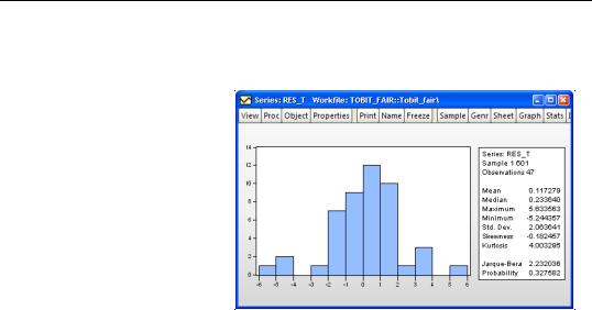
The histogram of the trimmed residual is depicted below.
This example illustrates the possibility that the number of observations that are lost by trimming can be quite large; out of the 601 observations in the sample, only 47 observations are left after trimming.
The tobit model imposes the restriction that the coefficients that determine the probability of being censored are the same as those that
determine the conditional mean of the uncensored observations. To test this restriction, we carry out the LR test by comparing the (restricted) tobit to the unrestricted log likelihood that is the sum of a probit and a truncated regression (we discuss truncated regression in detail in the following section). Save the tobit equation in the workfile by pressing the Name button, and enter a name, say EQ_TOBIT.
To estimate the probit, first create a dummy variable indicating uncensored observations by the command:
series y_c = (y_pt>0)
Then estimate a probit by replacing the dependent variable Y_PT by Y_C. A simple way to do this is to press Object/Copy Object… from the tobit equation toolbar. From the new untitled equation window that appears, press Estimate, edit the specification, replacing the dependent variable “Y_PT” with “Y_C”, choose Method: BINARY and click OK. Save the probit equation by pressing the Name button, say as EQ_BIN.
To estimate the truncated model, press Object/Copy Object… again from the tobit equation toolbar again. From the new untitled equation window that appears, press Estimate, mark the Truncated sample option, and click OK. Save the truncated regression by pressing the Name button, say as EQ_TR.
Then the LR test statistic and its p-value can be saved as a scalar by the commands:


 6
6