may use least squares to estimate an equation that explicitly includes the lags and leads of the cointegrating regressors.
Testing for Cointegration
In the single equation setting, EViews provides views that perform Engle and Granger (1987) and Phillips and Ouliaris (1990) residual-based tests, Hansen’s instability test (Hansen 1992b), and Park’s H(p, q) added variables test (Park 1992).
System cointegration testing using Johansen’s methodology is described in “Johansen Cointegration Test” on page 685.
Note that the Engle-Granger and Phillips-Perron tests may also be performed as a view of a Group object.
Residual-based Tests
The Engle-Granger and Phillips-Ouliaris residual-based tests for cointegration are simply unit root tests applied to the residuals obtained from SOLS estimation of Equation (25.1). Under the assumption that the series are not cointegrated, all linear combinations of
(yt, Xt¢), including the residuals from SOLS, are unit root nonstationary. Therefore, a test of the null hypothesis of no cointegration against the alternative of cointegration corresponds to a unit root test of the null of nonstationarity against the alternative of stationarity.
The two tests differ in the method of accounting for serial correlation in the residual series; the Engle-Granger test uses a parametric, augmented Dickey-Fuller (ADF) approach, while the Phillips-Ouliaris test uses the nonparametric Phillips-Perron (PP) methodology.
The Engle-Granger test estimates a p -lag augmented regression of the form
=
+
p
+ vt
ˆ
ˆ
ˆ
(25.17)
Du1t
(r – 1)u1t – 1
 dj Du1t – j
j = 1
The number of lagged differences p should increase to infinity with the (zero-lag) sample size T but at a rate slower than T1 § 3 .
We consider the two standard ADF test statistics, one based on the t-statistic for testing the null hypothesis of nonstationarity (r = 1) and the other based directly on the normalized autocorrelation coefficient rˆ – 1 :
ˆ
ˆ
=
r – 1
t
-------------
se
(r)
ˆ
ˆ
ˆ
(25.18)
=
T(r – 1)
z
--------------------------
ˆ
1
– Âdj
j
Testing for Cointegration—235
ˆ
ˆ
where se(r) is the usual OLS estimator of the standard error of the estimated
r
ˆ
=
ˆ
ˆ 2 –1 § 2
(25.19)
se(r)
sv
Âu1t – 1
t
(Stock 1986, Hayashi 2000). There is a practical question as to whether the standard error estimate in Equation (25.19) should employ a degree-of-freedom correction. Following common usage, EViews standalone unit root tests and the Engle-Granger cointegration tests both use the d.f.-corrected estimated standard error sˆv , with the latter test offering an option to turn off the correction.
In contrast to the Engle-Granger test, the Phillips-Ouliaris test obtains an estimate of r by running the unaugmented Dickey-Fuller regression
ˆ
=
ˆ
+ wt
(25.20)
Du1t
(r – 1)u1t – 1
and using the results to compute estimates of the long-run variance qw and the strict onesided long-run variance l1w of the residuals. By default, EViews d.f.-corrects the estimates of both long-run variances, but the correction may be turned off. (The d.f. correction employed in the Phillips-Ouliaris test differs slightly from the ones in FMOLS and CCR estimation since the former applies to the estimators of both long-run variances, while the latter apply only to the estimate of the conditional long-run variance).
The bias corrected autocorrelation coefficient is then given by
ˆ
=
ˆ
ˆ
ˆ
2
–1
(25.21)
(r – 1)
(r – 1) – Tl1w
Âu1t – 1
t
The test statistics corresponding to Equation (25.18) are
ˆ
r – 1
t
=
ˆ
----------------
(25.22)
se(r)
ˆ
– 1)
z = T(r
ˆ
ˆ
where
ˆ
=
ˆ
1 § 2
ˆ
2
–1 § 2
(25.23)
se(r)
qw
Âu1t – 1
t
As with ADF and PP statistics, the asymptotic distributions of the Engle-Granger and Phil- lips-Ouliaris z and t statistics are non-standard and depend on the deterministic regressors specification, so that critical values for the statistics are obtained from simulation results. Note that the dependence on the deterministics occurs despite the fact that the auxiliary regressions themselves exclude the deterministics (since those terms have already been removed from the residuals). In addition, the critical values for the ADF and PP test statistics must account for the fact that the residuals used in the tests depend upon estimated coefficients.
236—Chapter 25. Cointegrating Regression
MacKinnon (1996) provides response surface regression results for obtaining critical values for four different assumptions about the deterministic regressors in the cointegrating equation (none, constant (level), linear trend, quadratic trend) and values of k = m2 + 1 from 1 to 12. (Recall that m2 = max(n – p2, 0) is the number of cointegrating regressors less the number of deterministic trend regressors excluded from the cointegrating equation.)
When computing critical values, EViews will ignore the presence of any user-specified deterministic regressors since corresponding simulation results are not available. Furthermore, results for k = 12 will be used for cases that exceed that value.
Continuing with our consumption and income example from Hamilton, we construct EngleGranger and Phillips-Ouliaris tests from an estimated equation where the deterministic regressors include a constant and linear trend. Since SOLS is used to obtain the first-stage residuals, the test results do not depend on the method used to estimate the original equation, only the specification itself is used in constructing the test.
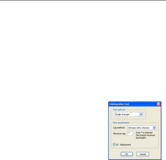
To perform the Engle-Granger test, open an estimated equation and select View/Cointegration and select Engle-Grangerin the Test Method combo. The dialog will change to display the options for this specifying the number p of augmenting lags in the ADF regression.
By default, EViews uses automatic lag-length selection using the Schwarz information criterion. The default number of lags is the observation-based rule given in Equation (25.16). Alternately you may specify a Fixed (User-specified)lag-length, select a different information criterion (Akaike, Hannan-Quinn, Modified Akaike, Modified Schwarz, or Modified HannanQuinn), or specify sequential testing of the highest order lag using a t-statistic and specified p-value threshold. For our purposes the default settings suffice so simply click on OK.
The Engle-Granger test results are divided into three
distinct sections. The first portion displays the test specification and settings, along with the test values and corresponding p-values:
Testing for Cointegration—237
Cointegration Test - Engle-Granger Date: 04/21/09 Time: 10:37 Equation: EQ_DOLS
Specification: LC LY C @TREND
Cointegrating equation deterministics: C @TREND Null hypothesis: Series are not cointegrated
Automatic lag specification (lag=1 based on Schwarz Info Criterion, maxlag=13)
Value
Prob.*
Engle-Granger tau-statistic
-4.536843
0.0070
Engle-Granger z-statistic
-33.43478
0.0108
*MacKinnon (1996) p-values.
The probability values are derived from the MacKinnon response surface simulation results. In settings where using the MacKinnon results may not be appropriate, for example when the cointegrating equation contains user-specified deterministic regressors or when there are more than 12 stochastic trends in the asymptotic distribution, EViews will display a warning message below these results.
Looking at the test description, we first confirm that the test statistic is computed using C and @TREND as deterministic regressors, and note that the choice to include a single lagged difference in the ADF regression was determined using automatic lag selection with a Schwarz criterion and a maximum lag of 13.
As to the tests themselves, the Engle-Granger tau-statistic (t-statistic)and normalized autocorrelation coefficient (which we term the z-statistic) both reject the null hypothesis of no cointegration (unit root in the residuals) at the 5% level. In addition, the tau-statistic rejects at a 1% significance level. On balance, the evidence clearly suggests that LC and LY are cointegrated.
The middle section of the output displays intermediate results used in constructing the test statistic that may be of interest:
Intermediate Results:
Rho - 1
-0.241514
Rho S.E.
0.053234
Residual variance
0.642945
Long-run residual variance
0.431433
Number of lags
1
Number of observations
169
Number of stochastic trends**
2
**Number of stochastic trends in asymptotic distribution.
Most of the entries are self-explanatory, though a few deserve a bit of discussion. First, the “Rho S.E.” and “Residual variance” are the (possibly) d.f. corrected coefficient standard error and the squared standard error of the regression. Next, the “Long-run residual variance” is the estimate of the long-run variance of the residual based on the estimated para-
238—Chapter 25. Cointegrating Regression
metric model. The estimator is obtained by taking the residual variance and dividing it by the square of 1 minus the sum of the lag difference coefficients. These residual variance and long-run variances are used to obtain the denominator of the z-statistic (Equation (25.18)). Lastly, the “Number of stochastic trends” entry reports the k = m2 + 1 value used to obtain the p-values. In the leading case, k is simply the number of cointegrating variables (including the dependent) in the system, but the value must generally account for deterministic trend terms in the system that are excluded from the cointegrating equation.
The bottom section of the output depicts the results for the actual ADF test equation:
Engle-Granger Test Equation:
Dependent Variable: D(RESID)
Method: Least Squares
Date: 04/21/09 Time: 10:37
Sample (adjusted): 1947Q3 1989Q3
Included observations: 169 after adjustments
Variable
Coefficient
Std. Error
t-Statistic
Prob.
RESID(-1)
-0.241514
0.053234
-4.536843
0.0000
D(RESID(-1))
-0.220759
0.071571
-3.084486
0.0024
R-squared
0.216944
Mean dependent var
-0.024433
Adjusted R-squared
0.212255
S.D. dependent var
0.903429
S.E. of regression
0.801838
Akaike info criterion
2.407945
Sum squared resid
107.3718
Schwarz criterion
2.444985
Log likelihood
-201.4713
Hannan-Quinn criter.
2.422976
Durbin-Watson stat
1.971405
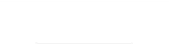
Alternately, you may compute the Phillips-Ouliaris test statistic. Simply select View/Cointegration and choose Phillips-Ouliarisin the Test Method combo.
The dialog changes to show a single Options button for controlling the estimation of the long-run variance qw and the strict one-sided long-run variance l1w . The default settings instruct EViews to compute these long-run variances using a non-prewhitened Bartlett kernel estimator with a fixed Newey-West bandwidth. To change these settings, click on the Options button and fill out the dialog. Since the default settings are sufficient for our needs, simply click on the OK button to compute the test statistics.
As before, the output may be divided into three parts; we will focus on the first two. The test results are given by:
qˆ 1w § 2
Testing for Cointegration—239
Cointegration Test - Phillips-Ouliaris Date: 04/21/09 Time: 10:40 Equation: EQ_DOLS
Specification: LC LY C @TREND
Cointegrating equation deterministics: C @TREND Null hypothesis: Series are not cointegrated
At the top of the output EViews notes that we estimated the long-run variance and onesided long run variance using a Bartlett kernel and an number of observations based bandwidth of 5.0. More importantly, the test statistics show that, as with the Engle-Granger tests, the Phillips-Ouliaris tests reject the null hypothesis of no cointegration (unit root in the residuals) at roughly the 1% significance level.
The intermediate results are given by:
Intermediate Results:
Rho - 1
-0.279221
Bias corrected Rho - 1 (Rho* - 1)
-0.256594
Rho* S.E.
0.050085
Residual variance
0.734699
Long-run residual variance
0.663836
Long-run residual autocovariance
-0.035431
Number of observations
170
Number of stochastic trends**
2
**Number of stochastic trends in asymptotic distribution.
There are a couple of new results. The “Bias corrected Rho - 1” reports the estimated value of Equation (25.21) and the “Rho* S.E.” corresponds to Equation (25.23). The “Long-run residual variance” and “Long-run residual autocovariance” are the estimates of qw and
l1w , respectively. It is worth noting that the ratio of to the S.E. of the regression, which is a measure of the amount of residual autocorrelation in the long-run variance, is the scaling factor used in adjusting the raw t-statistic to form tau.
The bottom portion of the output displays results for the test equation.
Hansen’s Instability Test
Hansen (1992) outlines a test of the null hypothesis of cointegration against the alternative of no cointegration. He notes that under the alternative hypothesis of no cointegration, one should expect to see evidence of parameter instability. He proposes (among others) use of the Lc test statistic, which arises from the theory of Lagrange Multiplier tests for parameter instability, to evaluate the stability of the parameters.
240—Chapter 25. Cointegrating Regression
The Lc statistic examines time-variation in the scores from the estimated equation. Let sˆt be the vector of estimated individual score contributions from the estimated equation, and define the partial sums,
t
ˆ
ˆ
St =
(25.24)
 st
r = 1
ˆ
= 0 by construction. For FMOLS, we have
where St
ˆ +
ˆ
ˆ +
¢
) –
l12
(25.25)
st =
(Zt ut
0
ˆ
+
+
ˆ
= y
– X
¢v is the residual for the transformed regression. Then Hansen
where u
t
t
t
ˆ
chooses a constant measure of the parameter instability G and forms the statistic
Lc =
T
ˆ
¢G
–1
ˆ
(25.26)
tr( Â St
St)
r = 1
For FMOLS, the natural estimator for G is
T
G =
ˆ
 ZtZt
¢
(25.27)
q1.2
t = 1
The sˆt and G may be defined analogously to least squares for CCR using the transformed data. For DOLS sˆt is defined for the subset of original regressors Zt , and G may be computed using the method employed in computing the original coefficient standard errors.
The distribution of Lc is nonstandard and depends on m2 = max(n – p2, 0), the number of cointegrating regressors less the number of deterministic trend regressors excluded from the cointegrating equation, and p the number of trending regressors in the system. Hansen (1992) has tabulated simulation results and provided polynomial functions allowing for computation of p-values for various values of m2 and p . When computing p-values, EViews ignores the presence of user-specified deterministic regressors in your equation.
In contrast to the residual based cointegration tests, Hansen’s test does rely on estimates from the original equation. We continue our illustration by considering an equation estimated on the consumption data using a constant and trend, FMOLS with a Quadratic Spectral kernel, Andrews automatic bandwidth selection, and no d.f. correction for the long-run variance and coefficient covariance estimates. The equation estimates are given by:
Testing for Cointegration—241
Dependent Variable: LC
Method: Fully Modified Least Squares (FMOLS) Date: 08/11/09 Time: 13:45
Sample (adjusted): 1947Q2 1989Q3 Included observations: 170 after adjustments
No d.f. adjustment for standard errors & covariance
Variable
Coefficient
Std. Error
t-Statistic
Prob.
LY
0.651766
0.057711
11.29361
0.0000
C
220.1345
37.89636
5.808855
0.0000
@TREND
0.289900
0.049542
5.851627
0.0000
R-squared
0.999098
Mean dependent var
720.5078
Adjusted R-squared
0.999087
S.D. dependent var
41.74069
S.E. of regression
1.261046
Sum squared resid
265.5695
Durbin-Watson stat
0.514132
Long-run variance
8.223497
There are no options for the Hansen test so you may simply click on View/Cointegration Tests..., select Hansen Instability in the combo box, then click on OK.
Cointegration Test - Hansen Parameter Instability Date: 08/11/09 Time: 13:48
Equation: EQ_19_3_31 Series: LC LY
Null hypothesis: Series are cointegrated Cointegrating equation deterministics: C
@TREND
No d.f. adjustment for score variance
Stochastic
Deterministic
Excluded
Lc statistic
Trends (m)
Trends (k)
Trends (p2)
Prob.*
0.575537
1
1
0
0.0641
*Hansen (1992b) Lc(m2=1, k=1) p-values, where m2=m-p2 is the number of stochastic trends in the asymptotic distribution
The top portion of the output describes the test hypothesis, the deterministic regressors, and any relevant information about the construction of the score variances. In this case, we see that the original equation had both C and @TREND as deterministic regressors, and that the score variance is based on the usual FMOLS variance with no d.f. correction.
The results are displayed below. The test statistic value of 0.5755 is presented in the first column. The next three columns describe the trends that determine the asymptotic distribution. Here there is a single stochastic regressor (LY) and one deterministic trend (@TREND) in the cointegrating equation, and no additional trends in the regressors equations. Lastly, we see from the final column that the Hansen test does not reject the null hypothesis that
242—Chapter 25. Cointegrating Regression
the series are cointegrated at conventional levels, though the relatively low p-value are cause for some concern, given the Engle-Granger and Phillips-Ouliaris results.
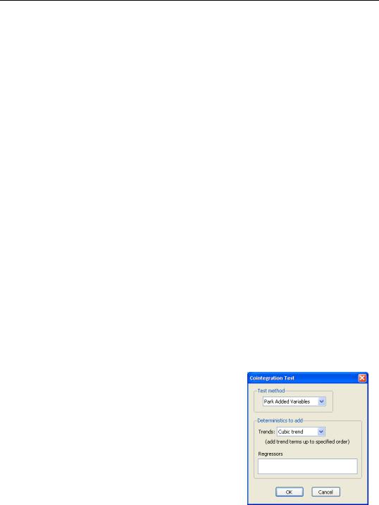
Park’s Added Variables Test
Park’s H(p, q) test is an added variable test. The test is computed by testing for the significance of spurious time trends in a cointegrating equation estimated using one of the methods described above.
Suppose we estimate equation Equation (25.1) where, to simplify, we let D1t consist solely of powers of trend up to order p . Then the Park test estimates the spurious regression model including from p + 1 to q spurious powers of trend
p
q
yt = Xt¢b + Â tsgs +
 tsgs + u1t
(25.28)
s =
0
s = p + 1
and tests for the joint significance of the coefficients (gp + 1, º, gq). Under the null hypothesis of cointegration, the spurious trend coefficients should be insignificant since the residual is stationary, while under the alternative, the spurious trend terms will mimic the remaining stochastic trend in the residual. Note that unless you wish to treat the constant as one of your spurious regressors, it should be included in the original equation specification.
Since the additional variables are simply deterministic regressors, we may apply a joint Wald test of significance to (gp + 1, º, gq). Under the maintained hypothesis that the original specification of the cointegrating equation is correct, the resulting test statistic is asymptotically x2q – p .
While one could estimate an equation with spurious trends and then to test for their significance using a Wald test, EViews offers a view which performs these steps for you. First estimate an equation where you include all trends that are assumed to be in the cointegrating equation. Next, select View/Cointegration Test... and choose Park Added Variables in the combo box. The dialog will change to allow you to specify the spurious trends.
There are two parts to the dialog. The combo box allows you to specify a trend polynomial. By default, the combo will be set to two orders higher than the trend order in the original equation. In our example equation which includes a linear trend, the default setting will include quadratic and cubic trend terms in the test equation and test for the significance of the two coefficients. You may use the edit field to enter non power-of-trend deterministic regressors.
We will use the default settings to perform a Park test on the FMOLS linear trend consumption equation con-