
- •Preface
- •Part IV. Basic Single Equation Analysis
- •Chapter 18. Basic Regression Analysis
- •Equation Objects
- •Specifying an Equation in EViews
- •Estimating an Equation in EViews
- •Equation Output
- •Working with Equations
- •Estimation Problems
- •References
- •Chapter 19. Additional Regression Tools
- •Special Equation Expressions
- •Robust Standard Errors
- •Weighted Least Squares
- •Nonlinear Least Squares
- •Stepwise Least Squares Regression
- •References
- •Chapter 20. Instrumental Variables and GMM
- •Background
- •Two-stage Least Squares
- •Nonlinear Two-stage Least Squares
- •Limited Information Maximum Likelihood and K-Class Estimation
- •Generalized Method of Moments
- •IV Diagnostics and Tests
- •References
- •Chapter 21. Time Series Regression
- •Serial Correlation Theory
- •Testing for Serial Correlation
- •Estimating AR Models
- •ARIMA Theory
- •Estimating ARIMA Models
- •ARMA Equation Diagnostics
- •References
- •Chapter 22. Forecasting from an Equation
- •Forecasting from Equations in EViews
- •An Illustration
- •Forecast Basics
- •Forecasts with Lagged Dependent Variables
- •Forecasting with ARMA Errors
- •Forecasting from Equations with Expressions
- •Forecasting with Nonlinear and PDL Specifications
- •References
- •Chapter 23. Specification and Diagnostic Tests
- •Background
- •Coefficient Diagnostics
- •Residual Diagnostics
- •Stability Diagnostics
- •Applications
- •References
- •Part V. Advanced Single Equation Analysis
- •Chapter 24. ARCH and GARCH Estimation
- •Basic ARCH Specifications
- •Estimating ARCH Models in EViews
- •Working with ARCH Models
- •Additional ARCH Models
- •Examples
- •References
- •Chapter 25. Cointegrating Regression
- •Background
- •Estimating a Cointegrating Regression
- •Testing for Cointegration
- •Working with an Equation
- •References
- •Binary Dependent Variable Models
- •Ordered Dependent Variable Models
- •Censored Regression Models
- •Truncated Regression Models
- •Count Models
- •Technical Notes
- •References
- •Chapter 27. Generalized Linear Models
- •Overview
- •How to Estimate a GLM in EViews
- •Examples
- •Working with a GLM Equation
- •Technical Details
- •References
- •Chapter 28. Quantile Regression
- •Estimating Quantile Regression in EViews
- •Views and Procedures
- •Background
- •References
- •Chapter 29. The Log Likelihood (LogL) Object
- •Overview
- •Specification
- •Estimation
- •LogL Views
- •LogL Procs
- •Troubleshooting
- •Limitations
- •Examples
- •References
- •Part VI. Advanced Univariate Analysis
- •Chapter 30. Univariate Time Series Analysis
- •Unit Root Testing
- •Panel Unit Root Test
- •Variance Ratio Test
- •BDS Independence Test
- •References
- •Part VII. Multiple Equation Analysis
- •Chapter 31. System Estimation
- •Background
- •System Estimation Methods
- •How to Create and Specify a System
- •Working With Systems
- •Technical Discussion
- •References
- •Vector Autoregressions (VARs)
- •Estimating a VAR in EViews
- •VAR Estimation Output
- •Views and Procs of a VAR
- •Structural (Identified) VARs
- •Vector Error Correction (VEC) Models
- •A Note on Version Compatibility
- •References
- •Chapter 33. State Space Models and the Kalman Filter
- •Background
- •Specifying a State Space Model in EViews
- •Working with the State Space
- •Converting from Version 3 Sspace
- •Technical Discussion
- •References
- •Chapter 34. Models
- •Overview
- •An Example Model
- •Building a Model
- •Working with the Model Structure
- •Specifying Scenarios
- •Using Add Factors
- •Solving the Model
- •Working with the Model Data
- •References
- •Part VIII. Panel and Pooled Data
- •Chapter 35. Pooled Time Series, Cross-Section Data
- •The Pool Workfile
- •The Pool Object
- •Pooled Data
- •Setting up a Pool Workfile
- •Working with Pooled Data
- •Pooled Estimation
- •References
- •Chapter 36. Working with Panel Data
- •Structuring a Panel Workfile
- •Panel Workfile Display
- •Panel Workfile Information
- •Working with Panel Data
- •Basic Panel Analysis
- •References
- •Chapter 37. Panel Estimation
- •Estimating a Panel Equation
- •Panel Estimation Examples
- •Panel Equation Testing
- •Estimation Background
- •References
- •Part IX. Advanced Multivariate Analysis
- •Chapter 38. Cointegration Testing
- •Johansen Cointegration Test
- •Single-Equation Cointegration Tests
- •Panel Cointegration Testing
- •References
- •Chapter 39. Factor Analysis
- •Creating a Factor Object
- •Rotating Factors
- •Estimating Scores
- •Factor Views
- •Factor Procedures
- •Factor Data Members
- •An Example
- •Background
- •References
- •Appendix B. Estimation and Solution Options
- •Setting Estimation Options
- •Optimization Algorithms
- •Nonlinear Equation Solution Methods
- •References
- •Appendix C. Gradients and Derivatives
- •Gradients
- •Derivatives
- •References
- •Appendix D. Information Criteria
- •Definitions
- •Using Information Criteria as a Guide to Model Selection
- •References
- •Appendix E. Long-run Covariance Estimation
- •Technical Discussion
- •Kernel Function Properties
- •References
- •Index
- •Symbols
- •Numerics

Chapter 25. Cointegrating Regression
This chapter describes EViews’ tools for estimating and testing single equation cointegrating relationships. Three fully efficient estimation methods, Fully Modified OLS (Phillips and Hansen 1992), Canonical Cointegrating Regression (Park 1992), and Dynamic OLS (Saikkonen 1992, Stock and Watson 1993) are described, along with various cointegration testing procedures: Engle and Granger (1987) and Phillips and Ouliaris (1990) residualbased tests, Hansen’s (1992b) instability test, and Park’s (1992) added variables test.
Notably absent from the discussion is Johansen’s (1991, 1995) system maximum likelihood approach to cointegration analysis and testing, which is supported using Var and Group objects, and fully documented in Chapter 32. “Vector Autoregression and Error Correction Models,” on page 459 and Chapter 38. “Cointegration Testing,” on page 685. Also excluded are single equation error correction methods which may be estimated using the Equation object and conventional OLS routines (see Phillips and Loretan (1991) for a survey).
The study of cointegrating relationships has been a particularly active area of research. We offer here an abbreviated discussion of the methods used to estimate and test for single equation cointegration in EViews. Those desiring additional detail will find a wealth of sources. Among the many useful overviews of literature are the textbook chapters in Hamilton (1994) and Hayashi (2000), the book length treatment in Maddala and Kim (1999), and the Phillips and Loretan (1991) and Ogaki (1993) survey articles.
Background
It is well known that many economic time series are difference stationary. In general, a regression involving the levels of these I(1) series will produce misleading results, with conventional Wald tests for coefficient significance spuriously showing a significant relationship between unrelated series (Phillips 1986).
Engle and Granger (1987) note that a linear combination of two or more I(1) series may be stationary, or I(0), in which case we say the series are cointegrated. Such a linear combination defines a cointegrating equation with cointegrating vector of weights characterizing the long-run relationship between the variables.
We will work with the standard triangular representation of a regression specification and assume the existence of a single cointegrating vector (Hansen 1992b, Phillips and Hansen
1990). Consider the n + 1 |
dimensional time series vector process (yt, Xt¢), with cointe- |
|
grating equation |
|
|
|
yt = Xt¢b + D1t¢g1 + u1t |
(25.1) |
where Dt = (D1t¢, D2t¢)¢ |
are deterministic trend regressors and the n stochastic regres- |
|
sors Xt are governed by the system of equations: |
|

220—Chapter 25. Cointegrating Regression
Xt = G21¢D1t + G22¢D2t + e2t
(25.2)
De2t = u2t
The p1 -vector of D1t regressors enter into both the cointegrating equation and the regressors equations, while the p2 -vector of D2t are deterministic trend regressors which are included in the regressors equations but excluded from the cointegrating equation (if a nontrending regressor such as the constant is present, it is assumed to be an element of D1t so it is not in D2t ).
Following Hansen (1992b), we assume that the innovations ut = (u1t, u2t¢)¢ are strictly stationary and ergodic with zero mean, contemporaneous covariance matrix S , one-sided long-run covariance matrix L , and nonsingular long-run covariance matrix Q , each of which we partition conformably with ut
S = E(u |
u ¢ ) = |
|
j11 j12 |
|
|
|
|
|
|
|||
t |
t |
|
S22 |
|
|
|
|
|
||||
|
|
|
j21 |
|
|
|
|
|
||||
• |
|
|
|
|
|
|
|
|
|
|
|
|
|
|
|
|
l11 |
l12 |
|
|
|||||
L = Â E(utut – j¢ ) = |
|
|
(25.3) |
|||||||||
j = 0 |
|
|
|
|
l21 |
L22 |
|
|
||||
• |
|
|
|
|
|
|
|
|
|
|
|
|
|
|
|
|
|
q11 q12 |
|
|
|||||
Q = Â E(utut – j¢) = |
|
|
= L + L¢ – S |
|
||||||||
j = –• |
|
|
q21 |
Q22 |
|
|
||||||
|
|
|
|
|||||||||
Taken together, the assumptions imply that the elements of yt and Xt |
are I(1) and cointe- |
grated but exclude both cointegration amongst the elements of Xt and multicointegration. Discussions of additional and in some cases alternate assumptions for this specification are provided by Phillips and Hansen (1990), Hansen (1992b), and Park (1992).
It is well-known that if the series are cointegrated, ordinary least squares estimation (static OLS) of the cointegrating vector b in Equation (25.1) is consistent, converging at a faster rate than is standard (Hamilton 1994). One important shortcoming of static OLS (SOLS) is that the estimates have an asymptotic distribution that is generally non-Gaussian, exhibit asymptotic bias, asymmetry, and are a function of non-scalar nuisance parameters. Since conventional testing procedures are not valid unless modified substantially, SOLS is generally not recommended if one wishes to conduct inference on the cointegrating vector.
The problematic asymptotic distribution of SOLS arises due to the presence of long-run correlation between the cointegrating equation errors and regressor innovations and(q12 ), and cross-correlation between the cointegrating equation errors and the regressors (l12). In the special case where the Xt are strictly exogenous regressors so that q12 = 0 and l12 = 0 , the bias, asymmetry, and dependence on non-scalar nuisance parameters vanish, and the

Estimating a Cointegrating Regression—221
SOLS estimator has a fully efficient asymptotic Gaussian mixture distribution which permits standard Wald testing using conventional limiting x2 -distributions.
Alternately, SOLS has an asymptotic Gaussian mixture distribution if the number of deterministic trends excluded from the cointegrating equation p2 is no less than the number of stochastic regressors n . Let m2 = max(n – p2, 0) represent the number of cointegrating regressors less the number of deterministic trend regressors excluded from the cointegrating equation. Then, roughly speaking, when m2 = 0 , the deterministic trends in the regressors asymptotically dominate the stochastic trend components in the cointegrating equation.
While Park (1992) notes that these two cases are rather exceptional, they are relevant in motivating the construction of our three asymptotically efficient estimators and computation of critical values for residual-based cointegration tests. Notably, the fully efficient estimation methods supported by EViews involve transformations of the data or modifications of the cointegrating equation specification to mimic the strictly exogenous Xt case.
Estimating a Cointegrating Regression
EViews offers three methods for estimating a single cointegrating vector: Fully Modified OLS (FMOLS), Canonical Cointegrating Regression (CCR), and Dynamic OLS (DOLS). Static OLS is supported as a special case of DOLS. We emphasize again that Johansen’s (1991, 1995) system maximum likelihood approach is discussed in Chapter 32. “Vector Autoregression and Error Correction Models,” on page 459.

222—Chapter 25. Cointegrating Regression
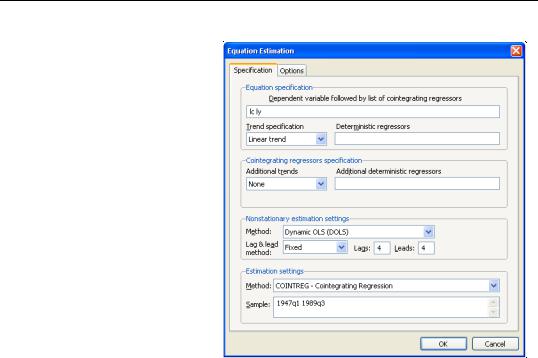
The equation object is used to estimate a cointegrating equation. First, create an equation object, select Object/New Object.../Equation or Quick/ Estimate Equation… then select COINTREG - Cointegrating Regression in the
Method combo box. The dialog will show settings appropriate for your cointegrating regression. Alternately, you may enter the cointreg keyword in the command window to perform both steps.
There are three parts to specifying your equation. First, you should use the first two sections of the dialog (Equation specification and Cointegrat-
ing regressors specification) to specify your triangular system of equations. Second, you will use the Nonstationary estimation settings section to specify the basic cointegrating regression estimation method. Lastly, you should enter a sample specification, then click on OK to estimate the equation. (We ignore, for a moment, the options settings on the Options tab.)
Specifying the Equation
The first two sections of the dialog (Equation specification and Cointegrating regressors specification) are used to describe your cointegrating and regressors equations.
Equation Specification
The cointegrating equation is described in the Equation specification section. You should enter the name of the dependent variable, y , followed by a list of cointegrating regressors, X , in the edit field, then use the Trend specification combo to choose from a

Estimating a Cointegrating Regression—223
list of deterministic trend variable assumptions (None, Constant (Level), Linear Trend, Quadratic Trend). The combo box selections imply trends up to the specified order so that the Quadratic Trend selection depicted includes a constant and a linear trend term along with the quadratic.
If you wish to add deterministic regressors that are not offered in the pre-specified list to D1 , you may enter the series names in the Deterministic regressors edit box.
Cointegrating Regressors Specification
Cointegrating Regressors Specification section of the dialog completes the specification of the regressors equations.
First, if there are any D2 deterministic trends (regressors that are included in the regressors equations but not in the cointegrating equation), they should be specified here using the Additional trends combo box or by entering regressors explicitly using the Additional deterministic regressors edit field.
Second, you should indicate whether you wish to estimate the regressors innovations u2t indirectly by estimating the regressors equations in levels and then differencing the residuals or directly by estimating the regressors equations in differences. Check the box for Estimate using differenced data (which is only relevant and only appears if you are estimating your equation using FMOLS or CCR) to estimate the regressors equations in differences.
Specifying an Estimation Method
Once you specify your cointegrating and regressor equations you are ready to describe your estimation method. The EViews equation object offers three methods for estimating a single cointegrating vector: Fully Modified OLS (FMOLS), Canonical Cointegrating Regression (CCR), and Dynamic OLS (DOLS). We again emphasize that Johansen’s (1991, 1995) system maximum likelihood approach is described elsewhere(“Vector Error Correction (VEC) Models” on page 478).
The Nonstationary estimation settings section is used to describe your estimation method. First, you should use the Method combo box to choose one of the three methods. Both the main dialog page and the options page will change to display the options associated with your selection.
Fully Modified OLS
Phillips and Hansen (1990) propose an estimator which employs a semi-parametric correction to eliminate the problems caused by the long run correlation between the cointegrating equation and stochastic regressors innovations. The resulting Fully Modified OLS (FMOLS) estimator is asymptotically unbiased and has fully efficient mixture normal asymptotics allowing for standard Wald tests using asymptotic Chi-square statistical inference.

224—Chapter 25. Cointegrating Regression
The FMOLS estimator employs preliminary estimates of the symmetric and one-sided long-
|
|
|
|
|
|
|
|
|
|
|
ˆ |
|
|
|
|
|
|
|
|
run covariance matrices of the residuals. Let u1t be the residuals obtained after estimating |
|||||||||||||||||||
|
|
|
|
ˆ |
|
|
|
|
|
|
|
|
ˆ |
|
|
ˆ |
|
from the levels regres- |
|
Equation (25.1). The u2t |
may be obtained indirectly as u2t |
= De2t |
|||||||||||||||||
sions |
|
|
|
|
|
|
|
|
|
|
|
|
|
|
|
|
|
|
|
|
|
|
|
|
Xt |
= |
ˆ |
|
|
|
ˆ |
|
ˆ |
|
|
|
|
|
(25.4) |
|
|
|
|
|
G21¢D1t |
+ G22¢D2t + e2t |
|
|
|
|
|
||||||||
or directly from the difference regressions |
|
|
|
|
|
|
|
|
|
|
|
||||||||
|
|
|
|
|
|
|
ˆ |
|
|
|
ˆ |
|
ˆ |
|
|
|
|
|
(25.5) |
|
|
|
|
|
DXt = G21¢DD1t + |
G22¢DD2t + u2t |
|
|
|
|
|||||||||
ˆ |
ˆ |
|
|
|
|
|
|
|
|
|
|
|
|
|
|
|
|
|
|
Let Q |
and L be the long-run covariance matrices computed using the residuals |
|
|||||||||||||||||
ˆ |
ˆ |
ˆ |
|
|
|
|
|
|
|
|
|
|
|
|
|
|
|
|
|
ut = |
(u1t, |
u2t¢)¢. Then we may define the modified data |
|
|
|
|
|
|
|||||||||||
|
|
|
|
|
|
+ |
= yt |
|
ˆ |
|
ˆ –1 |
ˆ |
|
|
|
|
|
|
|
|
|
|
|
|
|
yt |
|
|
|
|
|
|
|
|
|
(25.6) |
|||
|
|
|
|
|
|
|
– q12Q22 u2 |
|
|
|
|
|
|||||||
and an estimated bias correction term |
|
|
|
|
|
|
|
|
|
|
|
||||||||
|
|
|
|
|
ˆ + |
|
ˆ |
|
ˆ |
|
ˆ –1 |
ˆ |
|
|
|
|
|
(25.7) |
|
|
|
|
|
|
l12 |
= l12 |
– q12 |
Q22 |
L22 |
|
|
|
|
|
|||||
The FMOLS estimator is given by |
|
|
|
|
|
|
|
|
|
|
|
|
|
||||||
|
|
|
|
|
|
T |
|
|
|
–1 |
|
T |
|
|
|
|
|
|
|
|
|
|
|
ˆ |
|
|
|
|
|
|
ˆ |
+ |
|
|
|||||
|
|
ˆ |
|
|
|
|
|
|
|
+ |
|
¢ |
|
|
|||||
|
|
v |
= |
gˆ 1 |
= |
 Zt Zt¢ |
|
|
|
 Zt yt – |
T |
|
12 |
|
|
(25.8) |
|||
|
|
|
|
t = 1 |
|
|
|
t = 1 |
|
|
|
0 |
|
|
|
||||
|
|
|
|
|
|
||||||||||||||
where Zt = |
(Xt¢, Dt¢)¢. The key to FMOLS estimation is the construction of long-run |
||||||||||||||||||
|
|
|
|
|
ˆ |
|
|
ˆ |
|
|
|
|
|
|
|
|
|
|
|
covariance matrix estimators Q and L . |
|
|
|
|
|
|
|
|
|
|
|
|
|
|
|
ˆ |
ˆ |
Before describing the options available for computing Q and |
L , it |
||||
the scalar estimator |
|
|
|
|
|
ˆ |
= |
ˆ |
ˆ |
ˆ –1 ˆ |
|
q1.2 |
q11 |
– q12 |
Q22 q21 |
|
which may be interpreted as the estimated long-run variance of u1t may, if desired, apply a degree-of-freedom correction to qˆ 1.2 .
Hansen (1992) shows that the Wald statistic for the null hypothesis
W = |
ˆ |
|
|
ˆ |
–1 |
ˆ |
(Rv |
– r)¢(RV(v)R¢) |
|
(Rv – r) |
|||
with |
|
|
|
|
|
|
|
ˆ |
|
|
T |
|
–1 |
|
= |
ˆ |
 ZtZt¢ |
|||
|
V(v) |
q1.2 |
||||
|
|
|
|
t = 1 |
|
|
will be useful to define
(25.9)
conditional on u2t . We
Rv = r
(25.10)
(25.11)
has an asymptotic x2g -distribution, where g is the number of restrictions imposed by R . (You should bear in mind that restrictions on the constant term and any other non-trending variables are not testable using the theory underlying Equation (25.10).)

Estimating a Cointegrating Regression—225
To estimate your equation using FMOLS, select Fully-modified OLS (FMOLS) in the Nonstationary estimation settings combo box. The
main dialog and options pages will change to show the available settings.
To illustrate the FMOLS estimator, we employ data for (100 times) log real quarterly aggregate personal disposable income (LY) and personal consumption expenditures (LC) for the U.S. from 1947q1 to 1989q3 as described in Hamilton (2000, p. 600, 610) and contained in the workfile “Hamilton_coint.WF1”.
We wish to estimate a model that includes an intercept in the cointegrating equation, has no additional deterministics in the regressors equations, and estimates the regressors equations in non-differenced form.
By default, EViews will esti-
mate Q and L using a (non-prewhitened) kernel approach with a Bartlett kernel and Newey-West fixed bandwidth. To change the whitening or kernel settings, click on the Long-run variance calculation: Options button and enter your changes in the subdialog.

226—Chapter 25. Cointegrating Regression
Here we have specified that the long-run variances be computed using a nonparametric method with the Bartlett kernel and a real-valued bandwidth chosen by Andrews’ automatic bandwidth selection method.
In addition, you may use the Options tab of the Equation Estimation dialog to modify the computation of the coefficient covariance. By default, EViews computes the coefficient covariance by rescaling the usual OLS covariances using the qˆ 1.2
obtained from the estimated ˆ after applying a
Q degrees-of-freedom correction. In our example, we will use the checkbox on the Options tab (not depicted) to remove the d.f. correction.
The estimates for this specification are given by:
Dependent Variable: LC
Method: Fully Modified Least Squares (FMOLS) Date: 08/11/09 Time: 13:19
Sample (adjusted): 1947Q2 1989Q3 Included observations: 170 after adjustments Cointegrating equation deterministics: C
Long-run covariance estimate (Bartlett kernel, Andrews bandwidth = 14.9878)
No d.f. adjustment for standard errors & covariance
Variable |
Coefficient |
Std. Error |
t-Statistic |
Prob. |
|
|
|
|
|
|
|
|
|
|
LY |
0.987548 |
0.009188 |
107.4880 |
0.0000 |
C |
-0.035023 |
6.715362 |
-0.005215 |
0.9958 |
|
|
|
|
|
|
|
|
|
|
R-squared |
0.998171 |
Mean dependent var |
720.5078 |
|
Adjusted R-squared |
0.998160 |
S.D. dependent var |
41.74069 |
|
S.E. of regression |
1.790506 |
Sum squared resid |
538.5929 |
|
Durbin-Watson stat |
0.406259 |
Long-run variance |
25.46653 |
|
|
|
|
|
|
|
|
|
|
|
The top portion of the results describe the settings used in estimation, in particular, the specification of the deterministic regressors in the cointegrating equation, the kernel non-
parametric method used to compute the long-run variance estimators ˆ and ˆ , and the no-
Q L
d.f. correction option used in the calculation of the coefficient covariance. Also displayed is the bandwidth of 14.9878 selected by the Andrews automatic bandwidth procedure.
The estimated coefficients are presented in the middle of the output. Of central importance is the coefficient on LY which implies that the estimated cointegrating vector for LC and LY

Estimating a Cointegrating Regression—227
(1, -0.9875). Note that we present the standard error, t-statistic, and p-value for the constant even though they are not, strictly speaking, valid.
The summary statistic portion of the output is relatively familiar but does require a bit of comment. First, all of the descriptive and fit statistics are computed using the original data, not the FMOLS transformed data. Thus, while the measures of fit and the Durbin-Watson stat may be of casual interest, you should exercise extreme caution in using these measures. Second, EViews displays a “Long-run variance” value which is an estimate of the long-run variance of u1t conditional on u2t . This statistic, which takes the value of 25.47 in this
example, is the qˆ |
1.2 employed in forming the coefficient covariances, and is obtained from |
|
ˆ |
ˆ |
|
the Q and |
L used in estimation. Since we are not d.f. correcting the coefficient covariance |
matrix the qˆ 1.2 reported here is not d.f. corrected.
Once you have estimated your equation using FMOLS you may use the various cointegrating regression equation views and procedures. We will discuss these tools in greater depth in (“Working with an Equation” on page 243), but for now we focus on a simple Wald test for the coefficients. To test for whether the cointegrating vector is (1, -1), select View/Coefficient Diagnostics/Wald Test - Coefficient Restrictions and enter “C(1)=1” in the dialog. EViews displays the output for the test:
Wald Test:
Equation: FMOLS
Null Hypothesis: C(1)=1
Test Statistic |
Value |
df |
Probability |
|
|
|
|
|
|
|
|
t-statistic |
-1.355362 |
168 |
0.1771 |
F-statistic |
1.837006 |
(1, 168) |
0.1771 |
Chi-square |
1.837006 |
1 |
0.1753 |
|
|
|
|
|
|
|
|
Null Hypothesis Summary: |
|
|
|
|
|
|
|
|
|
|
|
Normalized Restriction (= 0) |
Value |
Std. Err. |
|
|
|
|
|
|
|
|
|
-1 + C(1) |
|
-0.012452 |
0.009188 |
|
|
|
|
|
|
|
|
Restrictions are linear in coefficients.
The t-statistic and Chi-square p-values are both around 0.17, indicating that the we cannot reject the null hypothesis that the cointegrating regressor coefficient value is equal to 1.
Note that this Wald test is for a simple linear restriction. Hansen points out that his theoretical results do not directly extend to testing nonlinear hypotheses in models with trend regressors, but EViews does allow tests with nonlinear restrictions since others, such as Phillips and Loretan (1991) and Park (1992) provide results in the absence of the trend regressors. We do urge caution in interpreting nonlinear restriction test results for equations involving such regressors.

228—Chapter 25. Cointegrating Regression
Canonical Cointegrating Regression
Park’s (1992) Canonical Cointegrating Regression (CCR) is closely related to FMOLS, but instead employs stationary transformations of the (y1t, Xt¢) data to obtain least squares estimates to remove the long run dependence between the cointegrating equation and stochastic regressors innovations. Like FMOLS, CCR estimates follow a mixture normal distribution which is free of non-scalar nuisance parameters and permits asymptotic Chi-square testing.
As in FMOLS, the first step in CCR is to obtain estimates of the innovations
uˆ t =ˆ (uˆ 1t, ˆuˆ 2t¢)¢ and corresponding consistent estimates of the long-run covariance matrices Q and L . Unlike FMOLS, CCR also requires a consistent estimator of the contempora-
neous covariance matrix ˆ .
S
|
|
|
|
|
|
ˆ |
|
|
|
|
|
|
||
Following Park, we extract the columns of L corresponding to the one-sided long-run cova- |
||||||||||||||
ˆ |
|
|
|
|
|
|
|
|
ˆ |
|
|
|
|
|
riance matrix of ut |
and (the levels and lags of) u2t |
|
|
|
|
|||||||||
|
|
|
|
ˆ |
|
|
|
ˆ |
|
|
|
|
|
|
|
|
|
|
|
|
|
|
|
|
|
|
|
||
|
|
|
|
= |
|
|
l12 |
|
|
|
|
|
(25.12) |
|
|
|
|
|
L2 |
|
|
ˆ |
|
|
|
|
|
||
|
|
|
|
|
|
|
|
L22 |
|
|
|
|
|
|
and transform the (y1t, Xt¢) |
using |
|
|
|
|
|
|
|
|
|
|
|||
|
Xt |
|
= |
ˆ |
–1 ˆ |
|
|
ˆ |
|
|
|
|
|
|
|
|
Xt – (S L2 ) |
¢ut |
|
|
|
|
|
|
|||||
|
|
|
|
|
|
|
|
|
|
|
|
|
|
(25.13) |
|
|
|
|
|
|
|
|
0 |
|
|||||
|
yt |
= |
ˆ –1 ˆ |
˜ |
|
|
|
ˆ |
||||||
|
|
yt – S L2 b + |
|
ˆ –1 |
ˆ |
|
|
¢ut |
||||||
|
|
|
|
|
|
|
|
|
|
Q22 |
q21 |
|
|
|
where the ˜ are estimates of the cointegrating equation coefficients, typically the SOLS esti- b
mates used to obtain the residuals uˆ 1t .
The CCR estimator is defined as ordinary least squares applied to the transformed data
ˆ
b gˆ 1
where Zt = (Zt ,¢D1t¢ )¢.
|
|
T |
–1 |
T |
|
= |
|
 Zt Zt ¢ |
|
 Zt yt |
(25.14) |
|
|
t = 1 |
|
t = 1 |
|
Park shows that the CCR transformations asymptotically eliminate the endogeneity caused by the long run correlation of the cointegrating equation errors and the stochastic regressors innovations, and simultaneously correct for asymptotic bias resulting from the contemporaneous correlation between the regression and stochastic regressor errors. Estimates based on the CCR are therefore fully efficient and have the same unbiased, mixture normal asymptotics as FMOLS. Wald testing may be carried out as in Equation (25.10) with Zt used in place of Zt in Equation (25.11).

Estimating a Cointegrating Regression—229
To estimate your equation using CCR, select Canonical Cointegrating Regression (CCR) in the Nonstationary estimation settings
combo box. The main dialog and options pages for CCR are identical to those for FMOLS.
To continue with our consumption and disposable income example, suppose we wish to estimate the same specification as before by CCR, using prewhitened Quadratic-spectral kernel estimators of the long-run covariance matrices. Fill out the equation specification portion of the dialog as before, then click on the Long-run variance calculation: Options button to change the calculation method. Here, we have specified a (fixed lag) VAR(1) for the prewhitening method and have changed our kernel shape to quadratic spectral. Click on OK to accept the covariance options
Once again go to the Options tab to turn off d.f. correction for the coefficient covariances so that
they match those from FMOLS. Click on OK again to accept the estimation options.
The results are presented below:
Dependent Variable: LC
Method: Canonical Cointegrating Regression (CCR) Date: 08/11/09 Time: 13:25
Sample (adjusted): 1947Q2 1989Q3 Included observations: 170 after adjustments Cointegrating equation deterministics: C
Long-run covariance estimate (Prewhitening with lags = 1, Quadratic -Spectral kernel, Andrews bandwidth = 1.5911)
No d.f. adjustment for standard errors & covariance
Variable |
Coefficient |
Std. Error |
t-Statistic |
Prob. |
|
|
|
|
|
|
|
|
|
|
LY |
0.988975 |
0.007256 |
136.3069 |
0.0000 |
C |
-1.958828 |
5.298819 |
-0.369673 |
0.7121 |
|
|
|
|
|
|
|
|
|
|
R-squared |
0.997780 |
Mean dependent var |
720.5078 |
|
Adjusted R-squared |
0.997767 |
S.D. dependent var |
41.74069 |
|
S.E. of regression |
1.972481 |
Sum squared resid |
653.6343 |
|
Durbin-Watson stat |
0.335455 |
Long-run variance |
15.91571 |
|
|
|
|
|
|
|
|
|
|
|
The first thing we note is that the VAR prewhitening has a strong effect on the kernel part of the calculation of the long-run covariances, shortening the Andrews optimal bandwidth

230—Chapter 25. Cointegrating Regression
from almost 15 down to 1.6. Furthermore, as a result of prewhitening, the estimate of the conditional long-run variance changes quite a bit, decreasing from 25.47 to 15.92. This decrease contributes to estimated coefficient standard errors for CCR that are smaller than their FMOLS counterparts. Differences aside, however, the estimates of the cointegrating vector are qualitatively similar. In particular, a Wald test of the null hypothesis that the cointegrating vector is equal to (1, -1) yields a p-value of 0.1305.
Dynamic OLS
A simple approach to constructing an asymptotically efficient estimator that eliminates the feedback in the cointegrating system has been advocated by Saikkonen (1992) and Stock and Watson (1993). Termed Dynamic OLS (DOLS), the method involves augmenting the cointegrating regression with lags and leads of DXt so that the resulting cointegrating equation error term is orthogonal to the entire history of the stochastic regressor innovations:
r |
|
yt = Xt¢b + D1t¢g1 + Â DXt +¢j d + v1t |
(25.15) |
j = –q
Under the assumption that adding q lags and r leads of the differenced regressors soaks up all of the long-run correlation between u1t and u2t , least-squares estimates of
v = (b¢, g¢)¢ using Equation (25.15) have the same asymptotic distribution as those obtained from FMOLS and CCR.
An estimator of the asymptotic variance matrix of ˆ may be computed by computing the v
usual OLS coefficient covariance, but replacing the usual estimator for the residual variance of v1t with an estimator of the long-run variance of the residuals. Alternately, you could compute a robust HAC estimator of the coefficient covariance matrix.
To estimate your equation using DOLS, first fill out the equation specification, then select
Dynamic OLS (DOLS) in the Nonstationary estimation settings combo box. The dialog will change to display settings for DOLS.
By default, the Lag & lead method is Fixed with Lags and Leads each set to 1. You may specify a different number of lags or leads or you can use the combo to elect auto-
matic information criterion selection of the lag and lead orders by selecting Akaike, Schwarz, or Hannan-Quinn. If you select None, EViews will estimate SOLS.
If you select one of the info criterion selection methods, you will be prompted for a maximum lag and lead length. You may enter a

Estimating a Cointegrating Regression—231
value, or you may retain the default entry “*” which instructs EViews to use an arbitrary observation-based rule-of-thumb:
int(min((T – k) § 3, 12) (T § 100)1 § 4 ) |
(25.16) |
to set the maximum, where k is the number of coefficients in the cointegrating equation. This rule-of-thumb is a slightly modified version of the rule suggested by Schwert (1989) in the context of unit root testing. (We urge careful thought in the use of automatic selection methods since the purpose of including leads and lags is to remove long-run dependence by orthogonalizing the equation residual with respect to the history of stochastic regressor innovations; the automatic methods were not designed to produce this effect.)
For DOLS estimation we may also specify the method used to compute the coefficient covariance matrix. Click on the Options tab of the dialog to see the relevant options.
The combo box allows you to choose between the Default (rescaled OLS), Ordinary Least Squares, White, or HAC - Newey West . The default computation method re-scales the ordinary least squares coefficient covariance using an estimator of the long-run variance of DOLS residuals (multiplying by the ratio of the long-run variance to the ordinary squared standard error). Alternately, you may employ a sandwichstyle HAC (Newey-West) covariance matrix estimator. In
both cases, the HAC Options button may be used to override the default method for computing the long-run variance (non-prewhitened Bartlett kernel and a Newey-West fixed bandwidth). In addition, EViews offers options for estimating the coefficient covariance using the White covariance or Ordinary Least Squares methods. These methods are offered primarily for comparison purposes.
Lastly, the Options tab may be used to remove the degree-of-freedom correction that is applied to the estimate of the conditional long-run variance or robust coefficient covariance.

232—Chapter 25. Cointegrating Regression
We illustrate the technique by estimating an example from Hamilton (19.3.31, p. 611) using the consumption and income data discussed earlier. The model employs an inter- cept-trend specification for the cointegrating equation, with no additional deterministics in the regressors equations, and four lags and leads of the differenced cointegrating regressor to eliminate long run correlation between the innovations.
Here, we have entered the cointegrating equation specification in the top portion of the dialog, and chosen Dynamic OLS (DOLS) as our estimation
method, and specified a Fixed lag and lead length of 4.
In computing the covariance matrix, Hamilton computes the long-run variance of the residuals using an AR(2) whitening regression with no d.f. correction. To match Hamilton’s computations, we click on the Options tab to display the covariance. First, turn off the adjustment for degrees of freedom by unchecking the d.f. Adjustment box. Next, with the combo set to Default (rescaled OLS), click on the HAC Options button to display the Longrun Variance Options dialog. Select a Fixed lag specification of 2, and choose the None kernel. Click on OK to accept the HAC settings, then on OK again to estimate the equation.
The estimation results are given below:

Estimating a Cointegrating Regression—233
Dependent Variable: LC |
|
|
|
|
Method: Dynamic Least Squares (DOLS) |
|
|
||
Date: 08/11/09 |
Time: 13:37 |
|
|
|
Sample (adjusted): 1948Q2 1988Q3 |
|
|
|
|
Included observations: 162 after adjustments |
|
|
||
Cointegrating equation deterministics: C @TREND |
|
|
||
Fixed leads and lags specification (lead=4, lag=4) |
|
|
||
Long-run variance estimate (Prewhitening with lags = 2, None kernel) |
||||
No d.f. adjustment for standard errors & covariance |
|
|
||
|
|
|
|
|
|
|
|
|
|
Variable |
Coefficient |
Std. Error |
t-Statistic |
Prob. |
|
|
|
|
|
|
|
|
|
|
LY |
0.681179 |
0.071981 |
9.463267 |
0.0000 |
C |
199.1406 |
47.20878 |
4.218297 |
0.0000 |
@TREND |
0.268957 |
0.062004 |
4.337740 |
0.0000 |
|
|
|
|
|
R-squared |
0.999395 |
Adjusted R-squared |
0.999351 |
S.E. of regression |
1.017016 |
Durbin-Watson stat |
0.422921 |
Mean dependent var |
720.5532 |
S.D. dependent var |
39.92349 |
Sum squared resid |
155.1484 |
Long-run variance |
10.19830 |
The top portion describes the settings used in estimation, showing the trend assumptions, the lag and lead specification, and method for computing the long-run variance used in forming the coefficient covariances. The actual estimate of the latter, in this case 10.198, is again displayed in the bottom portion of the output (if you had selected OLS as your coefficient covariance methods, this value would be simply be the ordinary S.E. of the regression; if you had selected White or HAC, the statistic would not have been computed).
The estimated coefficients are displayed in the middle of the output. First, note that EViews does not display the results for the lags and leads of the differenced cointegrating regressors since we cannot perform inference on these short-term dynamics nuisance parameters. Second, the coefficient on the linear trend is statistically different from zero at conventional levels, indicating that there is a deterministic time trend common to both LC and LY. Lastly, the estimated cointegrating vector for LC and LY is (1, -0.6812), which differs qualitatively from the earlier results. A Wald test of the restriction that the cointegrating vector is (1, -1) yields a t-statistic of -4.429, strongly rejecting that null hypothesis.
While EViews does not display the coefficients for the short-run dynamics, the short-run coefficients are used in constructing the fit statistics in the bottom portion of the results view (we again urge caution in using these measures). The short-run dynamics are also used in computing the residuals used by various equation views and procs such as the residual plot or the gradient view.
The short-run coefficients are not included in the representations view of the equation, which focuses only on the estimates for Equation (25.1). Furthermore, forecasting and model solution using an equation estimated by DOLS are also based on the long-run relationship. If you wish to construct forecasts that incorporate the short-run dynamics, you