

Examples—213
Examples
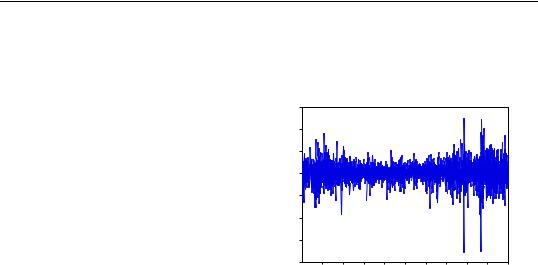
As an illustration of ARCH modeling in EViews, we estimate a model for the daily S&P 500 stock index from 1990 to 1999 (in the workfile “Stocks.WF1”). The dependent variable is the daily
continuously compounding return, log(st § st – 1 ), where st is the daily
close of the index. A graph of the return series clearly shows volatility clustering.
We will specify our mean equation with a simple constant:
|
|
|
|
DLOG(SPX) |
|
|
|
|
|
.06 |
|
|
|
|
|
|
|
|
|
.04 |
|
|
|
|
|
|
|
|
|
.02 |
|
|
|
|
|
|
|
|
|
.00 |
|
|
|
|
|
|
|
|
|
-.02 |
|
|
|
|
|
|
|
|
|
-.04 |
|
|
|
|
|
|
|
|
|
-.06 |
|
|
|
|
|
|
|
|
|
-.08 |
|
|
|
|
|
|
|
|
|
90 |
91 |
92 |
93 |
94 |
95 |
96 |
97 |
98 |
99 |
log(st § st – 1 ) = c1 + et |
(24.28) |
For the variance specification, we employ an EGARCH(1, 1) model:
2 |
) |
= |
2 |
|
et – 1 |
|
et – 1 |
(24.29) |
|
|
|||||||
log(jt |
q + blog(jt – 1 ) + a |
|
---------- |
|
+ g---------- |
|||
|
|
|
|
|
j |
|
jt – 1 |
|
|
|
|
|
|
t – 1 |
|
|
|
When we previously estimated a GARCH(1,1) model with the data, the standardized residual showed evidence of excess kurtosis. To model the thick tail in the residuals, we will assume that the errors follow a Student's t-distribution.
To estimate this model, open the GARCH estimation dialog, enter the mean specification:
dlog(spx) c
select the EGARCH method, enter 1 for the ARCH and GARCH orders and the Asymmetric order, and select Student’s t for the Error distribution. Click on OK to continue.
EViews displays the results of the estimation procedure. The top portion contains a description of the estimation specification, including the estimation sample, error distribution assumption, and backcast assumption.
Below the header information are the results for the mean and the variance equations, followed by the results for any distributional parameters. Here, we see that the relatively small degrees of freedom parameter for the t-distribution suggests that the distribution of the standardized errors departs significantly from normality.

214—Chapter 24. ARCH and GARCH Estimation
Dependent Variable: DLOG(SPX)
Method: ML - ARCH (Marquardt) - Student's t distribution
Date: 08/11/09 Time: 11:44
Sample: 1/02/1990 12/31/1999
Included observations: 2528
Convergence achieved after 30 iterations
Presample variance: backcast (parameter = 0.7)
LOG(GARCH) = C(2) + C(3)*ABS(RESID(-1)/@SQRT(GARCH(-1))) +
C(4)*RESID(-1)/@SQRT(GARCH(-1)) + C(5)*LOG(GARCH(-1))
Variable |
Coefficient |
Std. Error |
z-Statistic |
Prob. |
|
|
|
|
|
|
|
|
|
|
C |
0.000513 |
0.000135 |
3.810596 |
0.0001 |
|
|
|
|
|
|
|
|
|
|
|
Variance Equation |
|
|
|
|
|
|
|
|
C(2) |
-0.196710 |
0.039150 |
-5.024491 |
0.0000 |
C(3) |
0.113675 |
0.017550 |
6.477203 |
0.0000 |
C(4) |
-0.064068 |
0.011575 |
-5.535010 |
0.0000 |
C(5) |
0.988584 |
0.003360 |
294.2099 |
0.0000 |
|
|
|
|
|
|
|
|
|
|
T-DIST. DOF |
6.703689 |
0.844702 |
7.936156 |
0.0000 |
|
|
|
|
|
|
|
|
|
|
R-squared |
-0.000032 |
Mean dependent var |
0.000564 |
|
Adjusted R-squared |
-0.000032 |
S.D. dependent var |
0.008888 |
|
S.E. of regression |
0.008889 |
Akaike info criterion |
-6.871798 |
|
Sum squared resid |
0.199653 |
Schwarz criterion |
-6.857949 |
|
Log likelihood |
8691.953 |
Hannan-Quinn criter. |
-6.866773 |
|
Durbin-Watson stat |
1.963994 |
|
|
|
|
|
|
|
|
|
|
|
|
|
To test whether there any remaining ARCH effects in the residuals, select View/Residual Diagnostics/ARCH LM Test... and specify the order to test. Enter “7” in the dialog for the number of lags and click on OK. The top portion of the output from testing up-to an ARCH(7) is given by:
Heteroskedasticity Test: ARCH
F-statistic |
0.398894 |
Prob. F(7,2513) |
0.9034 |
Obs*R-squared |
2.798041 |
Prob. Chi-Square(7) |
0.9030 |
|
|
|
|
so there is little evidence of remaining ARCH effects.
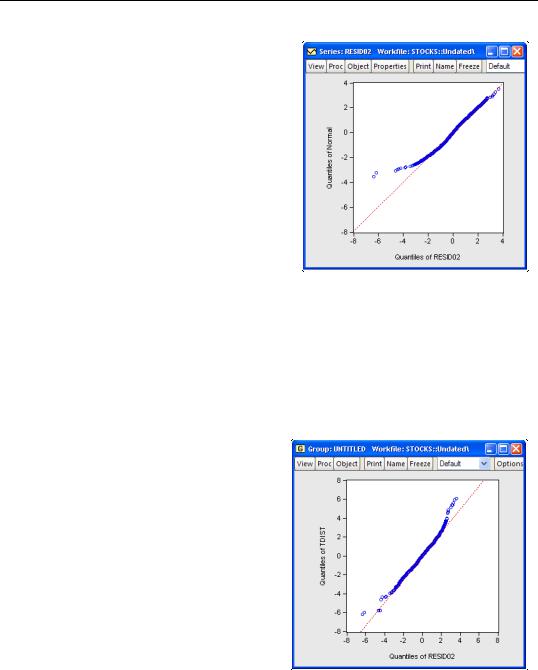
One way of further examining the distribution of the residuals is to plot the quantiles. First, save the standardized residuals by clicking on Proc/Make Residual Series..., select the Standardized option, and specify a name for the resulting series. EViews will create a series containing the desired residuals; in this example, we create a series named RESID02. Then open the residual series window and select View/Graph... and Quantile-Quantile/Theoret- ical from the list of graph types on the left-hand side of the dialog.
Examples—215
If the residuals are normally distributed, the points in the QQ-plots should lie alongside a straight line; see “Quantile-Quantile (Theoretical)” on page 507 of User’s Guide I for details on QQ-plots. The plot indicates that it is primarily large negative shocks that are driving the departure from normality. Note that we have modified the QQ-plot slightly by setting identical axes to facilitate comparison with the diagonal line.
We can also plot the residuals against the quantiles of the t-distribution. Instead of using the built-in QQ-plot for the t-distribu- tion, you could instead simulate a draw from a t-distribution and examine whether the
quantiles of the simulated observations match the quantiles of the residuals (this technique is useful for distributions not supported by EViews). The command:
series tdist = @qtdist(rnd, 6.7)
simulates a random draw from the t-distribution with 6.7 degrees of freedom. Then, create a group containing the series RESID02 and TDIST. Select View/Graph... and choose Quan- tile-Quantile from the left-hand side of the dialog and Empirical from the Q-Q graph dropdown on the right-hand side.
The large negative residuals more closely follow a straight line. On the other hand, one can see a slight deviation from t-distri- bution for large positive shocks. This is not unexpected, as the previous QQ-plot suggested that, with the exception of the large negative shocks, the residuals were close to normally distributed.
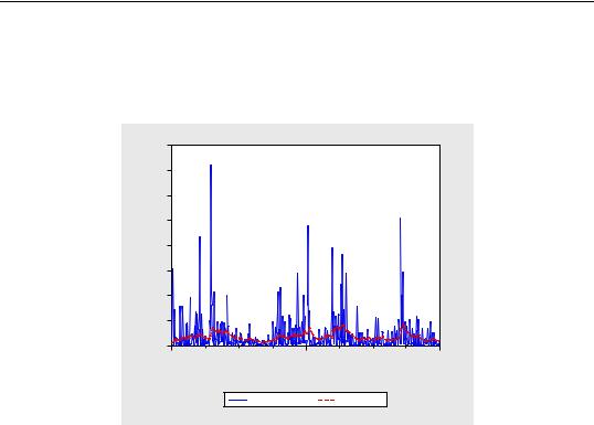
To see how the model might fit real data, we examine static forecasts for out-of-sam- ple data. Click on the Forecast button on the equation toolbar, type in “SPX_VOL” in the GARCH field to save the forecasted conditional variance, change the sample to the post-estimation sample period “1/1/2000
1/1/2002” and click on Static to select a static forecast.
216—Chapter 24. ARCH and GARCH Estimation
Since the actual volatility is unobserved, we will use the squared return series (DLOG(SPX)^2) as a proxy for the realized volatility. A plot of the proxy against the forecasted volatility provides an indication of the model’s ability to track variations in market volatility.
.0040 |
|
|
|
|
|
|
|
.0035 |
|
|
|
|
|
|
|
.0030 |
|
|
|
|
|
|
|
.0025 |
|
|
|
|
|
|
|
.0020 |
|
|
|
|
|
|
|
.0015 |
|
|
|
|
|
|
|
.0010 |
|
|
|
|
|
|
|
.0005 |
|
|
|
|
|
|
|
.0000 |
|
|
|
|
|
|
|
I |
II |
III |
IV |
I |
II |
III |
IV |
|
|
2000 |
|
|
2001 |
|
|
|
|
DLOG(SPX)^2 |
|
SPX_VOL |
|
|
|
References
Bollerslev, Tim (1986). “Generalized Autoregressive Conditional Heteroskedasticity,” Journal of Econometrics, 31, 307–327.
Bollerslev, Tim, Ray Y. Chou, and Kenneth F. Kroner (1992). “ARCH Modeling in Finance: A Review of the Theory and Empirical Evidence,” Journal of Econometrics, 52, 5–59.
Bollerslev, Tim, Robert F. Engle and Daniel B. Nelson (1994). “ARCH Models,” Chapter 49 in Robert F. Engle and Daniel L. McFadden (eds.), Handbook of Econometrics, Volume 4, Amsterdam: Elsevier Science B.V.
Bollerslev, Tim and Jeffrey M. Wooldridge (1992). “Quasi-Maximum Likelihood Estimation and Inference in Dynamic Models with Time Varying Covariances,” Econometric Reviews, 11, 143–172.
Ding, Zhuanxin, C. W. J. Granger, and R. F. Engle (1993). “A Long Memory Property of Stock Market Returns and a New Model,” Journal of Empirical Finance, 1, 83–106.
Engle, Robert F. (1982). “Autoregressive Conditional Heteroskedasticity with Estimates of the Variance of U.K. Inflation,” Econometrica, 50, 987–1008.
Engle, Robert F., and Bollerslev, Tim (1986). “Modeling the Persistence of Conditional Variances,” Econometric Reviews, 5, 1–50.
Engle, Robert F., David M. Lilien, and Russell P. Robins (1987). “Estimating Time Varying Risk Premia in the Term Structure: The ARCH-M Model,” Econometrica, 55, 391–407.
Glosten, L. R., R. Jaganathan, and D. Runkle (1993). “On the Relation between the Expected Value and the Volatility of the Normal Excess Return on Stocks,” Journal of Finance, 48, 1779–1801.

References—217
Nelson, Daniel B. (1991). “Conditional Heteroskedasticity in Asset Returns: A New Approach,” Econometrica, 59, 347–370.
Schwert, W. (1989). “Stock Volatility and Crash of ‘87,” Review of Financial Studies, 3, 77–102. Taylor, S. (1986). Modeling Financial Time Series, New York: John Wiley & Sons.
Zakoïan, J. M. (1994). “Threshold Heteroskedastic Models,” Journal of Economic Dynamics and Control, 18, 931-944.

218—Chapter 24. ARCH and GARCH Estimation