Chapter 24. ARCH and GARCH Estimation

196—Chapter 24. ARCH and GARCH Estimation

mation, it is called the conditional variance. The conditional variance equation specified in (24.2) is a function of three terms:

•A constant term: q .

•News about volatility from the previous period, measured as the lag of the squared residual from the mean equation: e2t – 1 (the ARCH term).

•Last period’s forecast variance: j2t – 1 (the GARCH term).

The (1, 1) in GARCH(1, 1) refers to the presence of a first-order autoregressive GARCH term (the first term in parentheses) and a first-order moving average ARCH term (the second term in parentheses). An ordinary ARCH model is a special case of a GARCH specification in which there are no lagged forecast variances in the conditional variance equation—i.e., a GARCH(0, 1).

This specification is often interpreted in a financial context, where an agent or trader predicts this period’s variance by forming a weighted average of a long term average (the constant), the forecasted variance from last period (the GARCH term), and information about volatility observed in the previous period (the ARCH term). If the asset return was unexpectedly large in either the upward or the downward direction, then the trader will increase the estimate of the variance for the next period. This model is also consistent with the volatility clustering often seen in financial returns data, where large changes in returns are likely to be followed by further large changes.

There are two equivalent representations of the variance equation that may aid you in interpreting the model:

•If we recursively substitute for the lagged variance on the right-hand side of Equation (24.2), we can express the conditional variance as a weighted average of all of the lagged squared residuals:

We see that the GARCH(1,1) variance specification is analogous to the sample variance, but that it down-weights more distant lagged squared errors.

•The error in the squared returns is given by ut = e2t – j2t . Substituting for the variances in the variance equation and rearranging terms we can write our model in

terms of the errors:

Thus, the squared errors follow a heteroskedastic ARMA(1,1) process. The autoregressive root which governs the persistence of volatility shocks is the sum of a plus b . In many applied settings, this root is very close to unity so that shocks die out rather slowly.

Basic ARCH Specifications—197

The GARCH(q, p) Model

Higher order GARCH models, denoted GARCH(q, p ), can be estimated by choosing either q or p greater than 1 where q is the order of the autoregressive GARCH terms and p is the order of the moving average ARCH terms.

The representation of the GARCH(q, p ) variance is:

The GARCH-M Model

The Xt in equation Equation (24.2) represent exogenous or predetermined variables that are included in the mean equation. If we introduce the conditional variance or standard deviation into the mean equation, we get the GARCH-in-Mean (GARCH-M) model (Engle, Lilien and Robins, 1987):

The ARCH-M model is often used in financial applications where the expected return on an asset is related to the expected asset risk. The estimated coefficient on the expected risk is a measure of the risk-return tradeoff.

Two variants of this ARCH-M specification use the conditional standard deviation or the log of the conditional variance in place of the variance in Equation (24.6).

Regressors in the Variance Equation

Equation (24.5) may be extended to allow for the inclusion of exogenous or predetermined regressors, z , in the variance equation:

Note that the forecasted variances from this model are not guaranteed to be positive. You may wish to introduce regressors in a form where they are always positive to minimize the possibility that a single, large negative value generates a negative forecasted value.

Distributional Assumptions

To complete the basic ARCH specification, we require an assumption about the conditional distribution of the error term e . There are three assumptions commonly employed when working with ARCH models: normal (Gaussian) distribution, Student’s t-distribution, and

198—Chapter 24. ARCH and GARCH Estimation

the Generalized Error Distribution (GED). Given a distributional assumption, ARCH models are typically estimated by the method of maximum likelihood.

For example, for the GARCH(1, 1) model with conditionally normal errors, the contribution

where j2t is specified in one of the forms above.

For the Student’s t-distribution, the log-likelihood contributions are of the form:

where the degree of freedom n > 2 controls the tail behavior. The t-distribution approaches the normal as n Æ •.

For the GED, we have:

By default, ARCH models in EViews are estimated by the method of maximum likelihood under the assumption that the errors are conditionally normally distributed.

Estimating ARCH Models in EViews

To estimate an ARCH or GARCH model, open the equation specification dialog by selecting

Quick/Estimate Equation…, by selecting Object/New Object.../Equation…. Select ARCH from the method combo box at the bottom of the dialog. Alternately, typing the keyword arch in the command line both creates the object and sets the estimation method.

The dialog will change to show you the ARCH specification dialog. You will need to specify both the mean and the variance specifications, the error distribution and the estimation sample.

200—Chapter 24. ARCH and GARCH Estimation

Variance regressors

In the Variance regressors edit box, you may optionally list variables you wish to include in the variance specification. Note that, with the exception of IGARCH models, EViews will always include a constant as a variance regressor so that you do not need to add C to this list.

The distinction between the permanent and transitory regressors is discussed in “The Component GARCH (CGARCH) Model” on page 211.

Restrictions

If you choose the GARCH/TARCH model, you may restrict the parameters of the GARCH model in two ways. One option is to set the Restrictions combo to IGARCH, which restricts the persistent parameters to sum up to one. Another is Variance Target, which restricts the constant term to a function of the GARCH parameters and the unconditional variance:

where jˆ 2 is the unconditional variance of the residuals.

The Error Distribution

To specify the form of the conditional distribution for your errors, you should select an entry from the Error Distribution combo box.You may choose between the default Normal (Gaussian), the Student’s t, the Generalized Error (GED), the Student’s t with fixed d.f., or the GED with fixed parameter. In the latter two cases, you will be prompted to enter a value for the fixed parameter. See “Distributional Assumptions” on page 197 for details on the supported distributions.

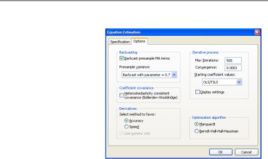
Estimation Options

EViews provides you with access to a number of optional estimation settings. Simply click on the Options tab and fill out the dialog as desired.

202—Chapter 24. ARCH and GARCH Estimation

Heteroskedasticity Consistent Covariances

Click on the check box labeled Heteroskedasticity Consistent Covariance to compute the quasi-maximum likelihood (QML) covariances and standard errors using the methods described by Bollerslev and Wooldridge (1992). This option is only available if you choose the conditional normal as the error distribution.

You should use this option if you suspect that the residuals are not conditionally normally distributed. When the assumption of conditional normality does not hold, the ARCH parameter estimates will still be consistent, provided the mean and variance functions are correctly specified. The estimates of the covariance matrix will not be consistent unless this option is specified, resulting in incorrect standard errors.

Note that the parameter estimates will be unchanged if you select this option; only the estimated covariance matrix will be altered.

Derivative Methods

EViews uses both numeric and analytic derivatives in estimating ARCH models. Fully analytic derivatives are available for GARCH(p, q) models with simple mean specifications assuming normal or unrestricted t-distribution errors.

Analytic derivatives are not available for models with ARCH in mean specifications, complex variance equation specifications (e.g. threshold terms, exogenous variance regressors, or integrated or target variance restrictions), models with certain error assumptions (e.g. errors following the GED or fixed parameter t-distributions), and all non-GARCH(p, q) models (e.g. EGARCH, PARCH, component GARCH).

Some specifications offer analytic derivatives for a subset of coefficients. For example, simple GARCH models with non-constant regressors allow for analytic derivatives for the variance coefficients but use numeric derivatives for any non-constant regressor coefficients.

You may control the method used in computing numeric derivatives to favor speed (fewer function evaluations) or to favor accuracy (more function evaluations).

Iterative Estimation Control

The likelihood functions of ARCH models are not always well-behaved so that convergence may not be achieved with the default estimation settings. You can use the options dialog to select the iterative algorithm (Marquardt, BHHH/Gauss-Newton), change starting values, increase the maximum number of iterations, or adjust the convergence criterion.

Starting Values

As with other iterative procedures, starting coefficient values are required. EViews will supply its own starting values for ARCH procedures using OLS regression for the mean equation. Using the Options dialog, you can also set starting values to various fractions of the

204—Chapter 24. ARCH and GARCH Estimation

Dependent Variable: DLOG(SPX)

Method: ML - ARCH (Marquardt) - Normal distribution Date: 08/11/09 Time: 10:57

Sample: 1/02/1990 12/31/1999 Included observations: 2528

Convergence achieved after 18 iterations Bollerslev-Wooldridge robust standard errors & covariance Presample variance: backcast (parameter = 0.7)

GARCH = C(2) + C(3)*RESID(-1)^2 + C(4)*GARCH(-1)

By default, the estimation output header describes the estimation sample, and the methods used for computing the coefficient standard errors, the initial variance terms, and the variance equation. Also noted is the method for computing the presample variance, in this case backcasting with smoothing parameter l = 0.7 .

The main output from ARCH estimation is divided into two sections—the upper part provides the standard output for the mean equation, while the lower part, labeled “Variance Equation”, contains the coefficients, standard errors, z-statistics and p-values for the coefficients of the variance equation.

The ARCH parameters correspond to a and the GARCH parameters to b in Equation (24.2) on page 195. The bottom panel of the output presents the standard set of regression statistics using the residuals from the mean equation. Note that measures such as R2 may not be meaningful if there are no regressors in the mean equation. Here, for example, the R2 is negative.

In this example, the sum of the ARCH and GARCH coefficients (a + b ) is very close to one, indicating that volatility shocks are quite persistent. This result is often observed in high frequency financial data.