

Stability Diagnostics—169
Heteroskedasticity Test: Harvey
F-statistic |
203.6910 |
Prob. F(10,324) |
0.0000 |
|
Obs*R-squared |
289.0262 |
Prob. Chi-Square(10) |
0.0000 |
|
Scaled explained SS |
160.8560 |
Prob. Chi-Square(10) |
0.0000 |
|
|
|
|
|
|
|
|
|
|
|
Test Equation: |
|
|
|
|
Dependent Variable: LRESID2 |
|
|
|
|
Method: Least Squares |
|
|
|
|
Date: 08/10/09 Time: 15:06 |
|
|
|
|
Sample (adjusted): 1959M07 1989M12 |
|
|
||
Included observations: 335 after adjustments |
|
|
||
|
|
|
|
|
|
|
|
|
|
Variable |
Coefficient |
Std. Error |
t-Statistic |
Prob. |
|
|
|
|
|
C |
2.320248 |
10.82443 |
0.214353 |
0.8304 |
LRESID2(-1) |
0.875599 |
0.055882 |
15.66873 |
0.0000 |
LRESID2(-2) |
0.061016 |
0.074610 |
0.817805 |
0.4141 |
LRESID2(-3) |
-0.035013 |
0.061022 |
-0.573768 |
0.5665 |
LRESID2(-6) |
0.024621 |
0.036220 |
0.679761 |
0.4971 |
LOG(IP) |
-1.622303 |
5.792786 |
-0.280056 |
0.7796 |
(LOG(IP))^2 |
0.255666 |
0.764826 |
0.334280 |
0.7384 |
(LOG(IP))*TB3 |
-0.040560 |
0.154475 |
-0.262566 |
0.7931 |
TB3 |
0.097993 |
0.631189 |
0.155252 |
0.8767 |
TB3^2 |
0.002845 |
0.005380 |
0.528851 |
0.5973 |
Y |
-0.023621 |
0.039166 |
-0.603101 |
0.5469 |
|
|
|
|
|
|
|
|
|
|
R-squared |
0.862765 |
Mean dependent var |
-4.046849 |
|
Adjusted R-squared |
0.858529 |
S.D. dependent var |
1.659717 |
|
S.E. of regression |
0.624263 |
Akaike info criterion |
1.927794 |
|
Sum squared resid |
126.2642 |
Schwarz criterion |
2.053035 |
|
Log likelihood |
-311.9056 |
Hannan-Quinn criter. |
1.977724 |
|
F-statistic |
203.6910 |
Durbin-Watson stat |
2.130511 |
|
Prob(F-statistic) |
0.000000 |
|
|
|
|
|
|
|
|
|
|
|
|
|
This output contains both the set of test statistics, and the results of the auxiliary regression on which they are based. All three statistics reject the null hypothesis of homoskedasticity.
Stability Diagnostics
EViews provides several test statistic views that examine whether the parameters of your model are stable across various subsamples of your data.
One common approach is to split the T observations in your data set of observations into T1 observations to be used for estimation, and T2 = T – T1 observations to be used for testing and evaluation. In time series work, you will usually take the first T1 observations for estimation and the last T2 for testing. With cross-section data, you may wish to order the data by some variable, such as household income, sales of a firm, or other indicator variables and use a subset for testing.
170—Chapter 23. Specification and Diagnostic Tests
Note that the alternative of using all available sample observations for estimation promotes a search for a specification that best fits that specific data set, but does not allow for testing predictions of the model against data that have not been used in estimating the model. Nor does it allow one to test for parameter constancy, stability and robustness of the estimated relationship.
There are no hard and fast rules for determining the relative sizes of T1 and T2 . In some cases there may be obvious points at which a break in structure might have taken place—a war, a piece of legislation, a switch from fixed to floating exchange rates, or an oil shock.
Where there is no reason a priori to expect a structural break, a commonly used rule-of- thumb is to use 85 to 90 percent of the observations for estimation and the remainder for testing.
EViews provides built-in procedures which facilitate variations on this type of analysis.
Chow's Breakpoint Test
The idea of the breakpoint Chow test is to fit the equation separately for each subsample and to see whether there are significant differences in the estimated equations. A
significant difference indicates a structural change in the relationship. For example, you can use this test to examine whether the demand function for energy was the same before and after the oil shock. The test may be used with least squares and two-stage least squares regressions; equations estimated using GMM offer a related test (see “GMM Breakpoint Test” on page 82).
By default the Chow breakpoint test tests whether there is a structural change in all of the equation parameters. However if the equation is linear EViews allows you to test whether there has been a structural change in a subset of the parameters.
To carry out the test, we partition the data into two or more subsamples. Each subsample must contain more observations than the number of coefficients in the equation so that the equation can be estimated. The Chow breakpoint test compares the sum of squared residuals obtained by fitting a single equation to the entire sample with the sum of squared residuals obtained when separate equations are fit to each subsample of the data.
EViews reports three test statistics for the Chow breakpoint test. The F-statistic is based on the comparison of the restricted and unrestricted sum of squared residuals and in the simplest case involving a single breakpoint, is computed as:
|
(u¢u – (u1¢u1 + u2¢u2)) § k |
|
F = |
˜ ˜ |
|
-----------------------------------------------------------------(u1¢u1 + u2¢u2) § (T – 2k)- , |
(23.25) |
|
˜ ˜ |
|
is the sum of squared residuals |
where u¢u is the restricted sum of squared residuals, ui¢ui |
||
from subsample i , T is the total number of observations, and k is the number of parame-
Stability Diagnostics—171
ters in the equation. This formula can be generalized naturally to more than one breakpoint. The F-statistic has an exact finite sample F-distribution if the errors are independent and identically distributed normal random variables.
The log likelihood ratio statistic is based on the comparison of the restricted and unrestricted maximum of the (Gaussian) log likelihood function. The LR test statistic has an asymptotic x2 distribution with degrees of freedom equal to (m – 1)k under the null hypothesis of no structural change, where m is the number of subsamples.
The Wald statistic is computed from a standard Wald test of the restriction that the coefficients on the equation parameters are the same in all subsamples. As with the log likelihood ratio statistic, the Wald statistic has an asymptotic x2 distribution with (m – 1)k degrees of freedom, where m is the number of subsamples.
One major drawback of the breakpoint test is that each subsample requires at least as many observations as the number of estimated parameters. This may be a problem if, for example, you want to test for structural change between wartime and peacetime where there are only a few observations in the wartime sample. The Chow forecast test, discussed below, should be used in such cases.
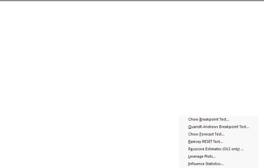
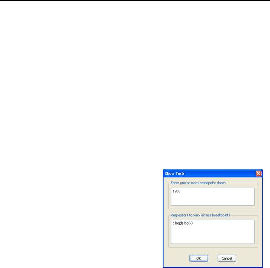
To apply the Chow breakpoint test, push View/
Stability Diagnostics/Chow Breakpoint Test… on the equation toolbar. In the dialog that appears, list the dates or observation numbers for the breakpoints in the upper edit field, and the regressors that are allowed to vary across breakpoints in the lower edit field.
For example, if your original equation was estimated from 1950 to 1994, entering:
1960
in the dialog specifies two subsamples, one from 1950 to 1959 and one from 1960 to 1994. Typing:
1960 1970
specifies three subsamples, 1950 to 1959, 1960 to 1969, and 1970 to 1994.
The results of a test applied to EQ1 in the workfile “Coef_test.WF1”, using the settings above are:

172—Chapter 23. Specification and Diagnostic Tests
Chow Breakpoint Test: 1960M01 1970M01
Null Hypothesis: No breaks at specified breakpoints
Varying regressors: All equation variables
Equation Sample: 1959M01 1989M12
F-statistic |
186.8638 |
Prob. F(6,363) |
0.0000 |
Log likelihood ratio |
523.8566 |
Prob. Chi-Square(6) |
0.0000 |
Wald Statistic |
1121.183 |
Prob. Chi-Square(6) |
0.0000 |
|
|
|
|
|
|
|
|
Indicating that the coefficients are not stable across regimes.
Quandt-Andrews Breakpoint Test
The Quandt-Andrews Breakpoint Test tests for one or more unknown structural breakpoints in the sample for a specified equation. The idea behind the Quandt-Andrews test is that a single Chow Breakpoint Test is performed at every observation between two dates, or observations, t1 and t2 . The k test statistics from those Chow tests are then summarized into one test statistic for a test against the null hypothesis of no breakpoints between t1 and t2 .
By default the test tests whether there is a structural change in all of the original equation parameters. For linear specifications, EViews also allows you to test whether there has been a structural change in a subset of the parameters.
From each individual Chow Breakpoint Test two statistics are retained, the Likelihood Ratio F-statistic and the Wald F-statistic. The Likelihood Ratio F-statistic is based on the comparison of the restricted and unrestricted sums of squared residuals. The Wald F-statistic is computed from a standard Wald test of the restriction that the coefficients on the equation parameters are the same in all subsamples. Note that in linear equations these two statistics will be identical. For more details on these statistics, see “Chow's Breakpoint Test” on page 170.
The individual test statistics can be summarized into three different statistics; the Sup or Maximum statistic, the Exp Statistic, and the Ave statistic (see Andrews, 1993 and Andrews and Ploberger, 1994). The Maximum statistic is simply the maximum of the individual Chow F-statistics:
MaxF = |
max |
(F(t)) |
|
(23.26) |
||
|
t1 |
£ t |
£ t2 |
|
|
|
The Exp statistic takes the form: |
|
|
|
|
|
|
ExpF = |
1 |
t2 |
exp |
1 |
|
(23.27) |
ln -- |
 |
--F(t) |
||||
|
k |
|
2 |
|
|
|
|
t = t1 |
|
|
|
|
|
The Ave statistic is the simple average of the individual F-statistics:
|
|
|
Stability Diagnostics—173 |
|
|
|
|
|
1 |
t2 |
|
AveF = |
--k |
 F(t) |
(23.28) |
|
|
t = t1 |
|
The distribution of these test statistics is non-standard. Andrews (1993) developed their true distribution, and Hansen (1997) provided approximate asymptotic p-values. EViews reports the Hansen p-values. The distribution of these statistics becomes degenerate as t1 approaches the beginning of the equation sample, or t2 approaches the end of the equation sample. To compensate for this behavior, it is generally suggested that the ends of the equation sample not be included in the testing procedure. A standard level for this “trimming” is 15%, where we exclude the first and last 7.5% of the observations. EViews sets trimming at 15% by default, but also allows the user to choose other levels. Note EViews only allows symmetric trimming, i.e. the same number of observations are removed from the beginning of the estimation sample as from the end.
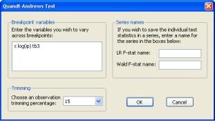
The Quandt-Andrews Breakpoint Test can be evaluated for an equation by selecting
View/Stability Diagnostics/ Quandt-Andrews Breakpoint Test… from the equation toolbar. The resulting dialog allows you to choose the level of symmetric observation trimming for the test, and, if your original equation was linear, which vari-
ables you wish to test for the unknown break point. You may also choose to save the individual Chow Breakpoint test statistics into new series within your workfile by entering a name for the new series.
As an example we estimate a consumption function, EQ1 in the workfile “Coef_test.WF1”, using annual data from 1947 to 1971. To test for an unknown structural break point amongst all the original regressors we run the Quandt-Andrews test with 15% trimming. This test gives the following results:
Note all three of the summary statistic measures fail to reject the null hypothesis of no structural breaks within the 17 possible dates tested. The maximum statistic was in 1962, and that is the most likely breakpoint location. Also, since the original equation was linear, note that the LR F-statistic is identical to the Wald F-statistic.

174—Chapter 23. Specification and Diagnostic Tests
Chow's Forecast Test
The Chow forecast test estimates two models—one using the full set of data T , and the other using a long subperiod T1 . Differences between the results for the two estimated models casts doubt on the stability of the estimated relation over the sample period. The Chow forecast test can be used with least squares and two-stage least squares regressions.
EViews reports two test statistics for the Chow forecast test. The F-statistic is computed as
|
|
(u¢u – u¢u) § T2 |
|
|
||
F |
= |
˜ |
˜ |
, |
(23.29) |
|
---------------------------------------u¢u § (T1 – k) |
||||||
|
|
|
|
|||
where u˜ ¢u˜ is the residual sum of squares when the equation is fitted to all T sample observations, u¢u is the residual sum of squares when the equation is fitted to T1 observations, and k is the number of estimated coefficients. This F-statistic follows an exact finite sample F-distribution if the errors are independent, and identically, normally distributed.
The log likelihood ratio statistic is based on the comparison of the restricted and unrestricted maximum of the (Gaussian) log likelihood function. Both the restricted and unrestricted log likelihood are obtained by estimating the regression using the whole sample. The restricted regression uses the original set of regressors, while the unrestricted regression adds a dummy variable for each forecast point. The LR test statistic has an asymptotic
x2 distribution with degrees of freedom equal to the number of forecast points T2 under the null hypothesis of no structural change.
To apply Chow’s forecast test, push View/Stability Diagnostics/Chow Forecast Test… on the equation toolbar and specify the date or observation number for the beginning of the forecasting sample. The date should be within the current sample of observations.
As an example, using the “Coef_test2.WF1” workfile, suppose we estimate a consumption function, EQ1, using quarterly data from 1947q1 to 1994q4 and specify 1973q1 as the first observation in the forecast period. The test reestimates the equation for the period 1947q1 to 1972q4, and uses the result to compute the prediction errors for the remaining quarters, and the top portion of the table shows the following results:

Stability Diagnostics—175
Chow Forecast Test
Equation: EQ1
Specification: LOG(CS) C LOG(GDP)
Test predictions for observations from 1973Q1 to 1994:4
|
Value |
df |
Probability |
|
F-statistic |
0.708348 |
(88, 102) |
0.9511 |
|
Likelihood ratio |
91.57087 |
88 |
0.3761 |
|
|
|
|
|
|
|
|
|
|
|
F-test summary: |
|
|
Mean |
|
|
|
|
|
|
|
Sum of Sq. |
df |
Squares |
|
Test SSR |
0.061798 |
88 |
0.000702 |
|
Restricted SSR |
0.162920 |
190 |
0.000857 |
|
Unrestricted SSR |
0.101122 |
102 |
0.000991 |
|
Unrestricted SSR |
0.101122 |
102 |
0.000991 |
|
|
|
|
|
|
|
|
|
|
|
LR test summary: |
Value |
df |
|
|
|
|
|
||
Restricted LogL |
406.4749 |
190 |
|
|
Unrestricted LogL |
452.2603 |
102 |
|
|
|
|
|
|
|
|
|
|
|
|
Unrestricted log likelihood adjusts test equation results to account for observations in forecast sample
Neither of the forecast test statistics reject the null hypothesis of no structural change in the consumption function before and after 1973q1.
If we test the same hypothesis using the Chow breakpoint test, the result is:
Chow Breakpoint Test: 1973Q1
Null Hypothesis: No breaks at specified breakpoints
Varying regressors: All equation variables
Equation Sample: 1947Q1 1994Q4
F-statistic |
38.39198 |
Prob. F(2,188) |
0.0000 |
Log likelihood ratio |
65.75466 |
Prob. Chi-Square(2) |
0.0000 |
Wald Statistic |
76.78396 |
Prob. Chi-Square(2) |
0.0000 |
|
|
|
|
|
|
|
|
Note that the breakpoint test statistics decisively reject the hypothesis from above. This example illustrates the possibility that the two Chow tests may yield conflicting results.
Ramsey's RESET Test
RESET stands for Regression Specification Error Test and was proposed by Ramsey (1969). The classical normal linear regression model is specified as:
y = Xb + e , |
(23.30) |
where the disturbance vector e is presumed to follow the multivariate normal distribution N(0, j2I). Specification error is an omnibus term which covers any departure from the assumptions of the maintained model. Serial correlation, heteroskedasticity, or non-normal-

176—Chapter 23. Specification and Diagnostic Tests
ity of all violate the assumption that the disturbances are distributed N(0, j2I) . Tests for these specification errors have been described above. In contrast, RESET is a general test for the following types of specification errors:
•Omitted variables; X does not include all relevant variables.
•Incorrect functional form; some or all of the variables in y and X should be transformed to logs, powers, reciprocals, or in some other way.
•Correlation between X and e , which may be caused, among other things, by measurement error in X , simultaneity, or the presence of lagged y values and serially
correlated disturbances.
Under such specification errors, LS estimators will be biased and inconsistent, and conventional inference procedures will be invalidated. Ramsey (1969) showed that any or all of these specification errors produce a non-zero mean vector for e . Therefore, the null and alternative hypotheses of the RESET test are:
H0: e ~ N(0, j2I) |
|
(23.31) |
H1: e ~ N(m, j2I) |
|
|
m π 0 |
|
|
The test is based on an augmented regression: |
|
|
y = Xb + Zg + e . |
(23.32) |
|
The test of specification error evaluates the restriction g = 0 . The crucial question in constructing the test is to determine what variables should enter the Z matrix. Note that the Z matrix may, for example, be comprised of variables that are not in the original specification, so that the test of g = 0 is simply the omitted variables test described above.
In testing for incorrect functional form, the nonlinear part of the regression model may be some function of the regressors included in X . For example, if a linear relation,
y = b0 + b1X + e , |
(23.33) |
is specified instead of the true relation: |
|
y = b0 + b1X + b2X2 + e |
(23.34) |
the augmented model has Z = X2 and we are back to the omitted variable case. A more general example might be the specification of an additive relation,
y = b0 + b1X1 + b2X2 + e |
(23.35) |
instead of the (true) multiplicative relation: |
|
y = b0X1b1 X2b2 + e . |
(23.36) |

Stability Diagnostics—177
A Taylor series approximation of the multiplicative relation would yield an expression involving powers and cross-products of the explanatory variables. Ramsey's suggestion is to include powers of the predicted values of the dependent variable (which are, of course, linear combinations of powers and cross-product terms of the explanatory variables) in Z :
Z = |
ˆ 2 |
ˆ 3 |
ˆ |
4 |
, º] |
(23.37) |
[y |
, y |
, y |
|
|||
ˆ |
|
|
|
|
|
y on X . The superscripts indi- |
where y is the vector of fitted values from the regression of |
||||||
cate the powers to which these predictions are raised. The first power is not included since it is perfectly collinear with the X matrix.
Output from the test reports the test regression and the F-statistic and log likelihood ratio for testing the hypothesis that the coefficients on the powers of fitted values are all zero. A study by Ramsey and Alexander (1984) showed that the RESET test could detect specification error in an equation which was known a priori to be misspecified but which nonetheless gave satisfactory values for all the more traditional test criteria—goodness of fit, test for first order serial correlation, high t-ratios.
To apply the test, select View/Stability Diagnostics/Ramsey RESET Test… and specify the number of fitted terms to include in the test regression. The fitted terms are the powers of the fitted values from the original regression, starting with the square or second power. For example, if you specify 1, then the test will add yˆ 2 in the regression, and if you specify 2, then the test will add yˆ 2 and yˆ 3 in the regression, and so on. If you specify a large number of fitted terms, EViews may report a near singular matrix error message since the powers of the fitted values are likely to be highly collinear. The Ramsey RESET test is only applicable to equations estimated using selected methods.
Recursive Least Squares
In recursive least squares the equation is estimated repeatedly, using ever larger subsets of the sample data. If there are k coefficients to be estimated in the b vector, then the first k observations are used to form the first estimate of b . The next observation is then added to the data set and k + 1 observations are used to compute the second estimate of b . This process is repeated until all the T sample points have been used, yielding T – k + 1 estimates of the b vector. At each step the last estimate of b can be used to predict the next value of the dependent variable. The one-step ahead forecast error resulting from this prediction, suitably scaled, is defined to be a recursive residual.
More formally, let Xt – 1 denote the (t – 1) ¥ k matrix of the regressors from period 1 to period t – 1 , and yt – 1 the corresponding vector of observations on the dependent variable. These data up to period t – 1 give an estimated coefficient vector, denoted by bt – 1 . This coefficient vector gives you a forecast of the dependent variable in period t . The forecast is xt¢bt – 1 , where xt¢ is the row vector of observations on the regressors in period t . The forecast error is yt – xt¢bt – 1 , and the forecast variance is given by:
178—Chapter 23. Specification and Diagnostic Tests
|
j2(1 + xt¢(Xt – 1¢Xt – 1 )–1xt). |
|
|
(23.38) |
|||
The recursive residual wt |
is defined in EViews as: |
|
|
|
|
||
wt |
= |
(yt – xt – 1¢b) |
|
|
. |
(23.39) |
|
(-----------------------------------------------------------------------1 + xt¢(Xt – 1¢Xt – 1)–1xt) |
1 |
§ 2 |
|||||
|
|
|
|
||||
These residuals can be computed for t = k + 1, º, T . If the maintained model is valid, the recursive residuals will be independently and normally distributed with zero mean and constant variance j2 .
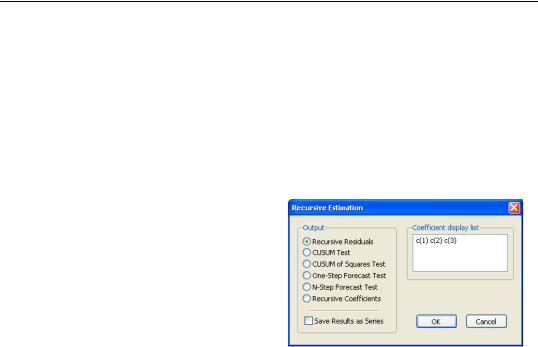
To calculate the recursive residuals, press
View/Stability Diagnostics/Recursive Estimates (OLS only)… on the equation toolbar. There are six options available for the recursive estimates view. The recursive estimates view is only available for equations estimated by ordinary least squares without AR and MA terms. The Save Results as Series option allows you to save the recursive residuals and recursive
coefficients as named series in the workfile; see “Save Results as Series” on page 181.
Recursive Residuals
This option shows a plot of the recursive residuals about the zero line. Plus and minus two standard errors are also shown at each point. Residuals outside the standard error bands suggest instability in the parameters of the equation.
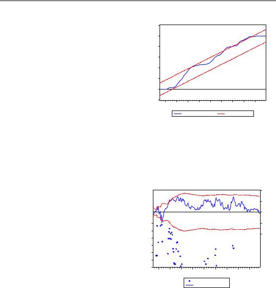
CUSUM Test
The CUSUM test (Brown, Durbin, and Evans, 1975) is based on the cumulative sum of the recursive residuals. This option plots the cumulative sum together with the 5% critical lines. The test finds parameter instability if the cumulative sum goes outside the area between the two critical lines.
The CUSUM test is based on the statistic:
t |
|
Wt = Â wr § s , |
(23.40) |
r = k + 1
for t = k + 1, º, T , where w is the recursive residual defined above, and s is the standard deviation of the recursive residuals wt . If the b vector remains constant from period to period, E(Wt) = 0 , but if b changes, Wt will tend to diverge from the zero mean value line. The significance of any departure from the zero line is assessed by reference to a
Stability Diagnostics—179
pair of 5% significance lines, the distance between which increases with t . The 5% significance lines are found by connecting the points:
[k, ±–0.948(T – k)1 § 2] |
and |
[T, ±3 ¥ 0.948(T – k)1 § 2]. |
(23.41) |
Movement of Wt outside the critical lines is suggestive of coefficient instability. A sample CUSUM is given below:
300 |
|
|
|
|
|
|
|
|
250 |
|
|
|
|
|
|
|
|
200 |
|
|
|
|
|
|
|
|
150 |
|
|
|
|
|
|
|
|
100 |
|
|
|
|
|
|
|
|
50 |
|
|
|
|
|
|
|
|
0 |
|
|
|
|
|
|
|
|
-50 |
|
|
|
|
|
|
|
|
50 |
55 |
60 |
65 |
70 |
75 |
80 |
85 |
90 |
|
|
CUSUM |
5% Significance |
|
|
The test clearly indicates instability in the equation during the sample period.
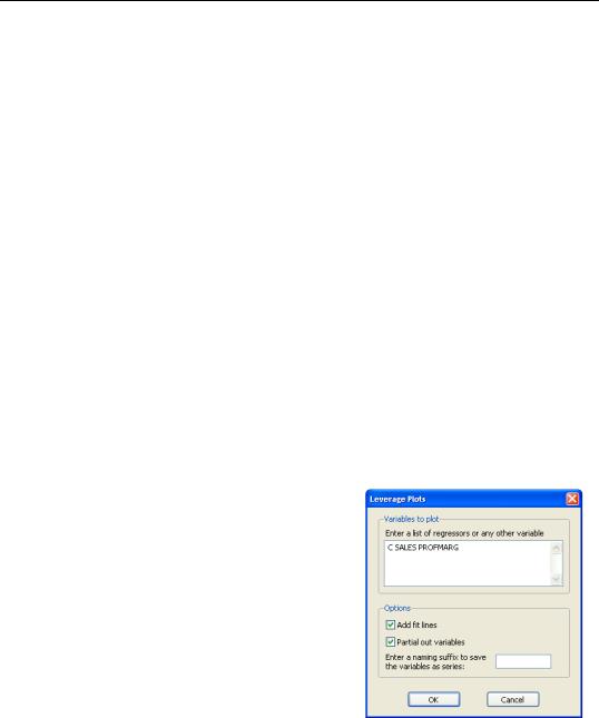
CUSUM of Squares Test
The CUSUM of squares test (Brown, Durbin, and Evans, 1975) is based on the test statistic:
|
|
t |
|
|
T |
|
|
St = |
 |
wr2 |
§ |
 |
wr2 . |
(23.42) |
|
|
|
r = k + 1 |
|
r = k + 1 |
|
|
|
The expected value of St |
under the hypothesis of parameter constancy is: |
|
|||||
|
E(St) = |
(t – k) § (T – k) |
(23.43) |
||||
which goes from zero at t |
= k to unity at t |
= T . The significance of the departure of S |
|||||
from its expected value is assessed by reference to a pair of parallel straight lines around the expected value. See Brown, Durbin, and Evans (1975) or Johnston and DiNardo (1997, Table D.8) for a table of significance lines for the CUSUM of squares test.
The CUSUM of squares test provides a plot of St against t and the pair of 5 percent critical lines. As with the CUSUM test, movement outside the critical lines is suggestive of parameter or variance instability.
180—Chapter 23. Specification and Diagnostic Tests
The cumulative sum of squares is generally within the 5% significance lines, suggesting that the residual variance is somewhat stable.
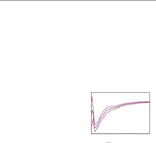
One-Step Forecast Test
If you look back at the definition of the recursive residuals given above, you will see that each recursive residual is the error
in a one-step ahead forecast. To test whether the value of the dependent variable at time t might have come from the
model fitted to all the data up to that point,
each error can be compared with its standard deviation from the full sample.
The One-Step Forecast Test option produces a plot of the recursive residuals and standard errors and the sample points whose probability value is at or below 15 percent. The plot can help you spot the periods when your equation is least successful. For example, the one-step ahead forecast test might look like this:
The upper portion of the plot (right vertical axis) repeats the recursive residuals and standard errors displayed by the
Recursive Residuals option. The lower portion of the plot (left vertical axis) shows the probability values for those sample points where the hypothesis of parameter constancy would be rejected at the 5, 10, or 15 percent levels. The points with p-values less the 0.05 correspond to those points where the recursive residuals go outside the two standard error bounds.
|
|
|
|
|
|
|
|
.08 |
|
|
|
|
|
|
|
|
.04 |
|
|
|
|
|
|
|
|
.00 |
.000 |
|
|
|
|
|
|
|
-.04 |
.025 |
|
|
|
|
|
|
|
-.08 |
.050 |
|
|
|
|
|
|
|
|
|
|
|
|
|
|
|
|
|
.075 |
|
|
|
|
|
|
|
|
.100 |
|
|
|
|
|
|
|
|
.125 |
|
|
|
|
|
|
|
|
.150 |
|
|
|
|
|
|
|
|
50 |
55 |
60 |
65 |
70 |
75 |
80 |
85 |
90 |
One-Step Probability
Recursive Residuals
For the test equation, there is evidence of instability early in the sample period.
N-Step Forecast Test
This test uses the recursive calculations to carry out a sequence of Chow Forecast tests. In contrast to the single Chow Forecast test described earlier, this test does not require the specification of a forecast period— it automatically computes all feasible cases, starting with the smallest possible sample size for estimating the forecasting equation and then adding
Stability Diagnostics—181
one observation at a time. The plot from this test shows the recursive residuals at the top and significant probabilities (based on the F-statistic) in the lower portion of the diagram.
Recursive Coefficient Estimates
This view enables you to trace the evolution of estimates for any coefficient as more and more of the sample data are used in the estimation. The view will provide a plot of selected coefficients in the equation for all feasible recursive estimations. Also shown are the two standard error bands around the estimated coefficients.
If the coefficient displays significant variation as more data is added to the estimating equation, it is a strong indication of instability. Coefficient plots will sometimes show dramatic jumps as the postulated equation tries to digest a structural break.
To view the recursive coefficient estimates, click the Recursive Coefficients option and list the coefficients you want to plot in the Coefficient Display List field of the dialog box. The recursive estimates of the marginal propensity to consume (coefficient C(2)), from the sample consumption function are provided below:
The estimated propensity to consume rises steadily as we add more data over the sample period, approaching a value of one.
Save Results as Series
1.3
1.2
1.1 
1.0
0.9
0.8
The Save Results as Series checkbox will |
0.7 |
|
do different things depending on the plot |
||
0.6 |
||
you have asked to be displayed. When |
||
0.5 |
||
paired with the Recursive Coefficients |
||
0.4 |
option, Save Results as Series will instruct |
50 |
55 |
60 |
65 |
70 |
75 |
80 |
85 |
90 |
||
|
|
|
|
|
|
|
|
|
|
|
|
|
|
|
|
|
|
|
|
|
|||
EViews to save all recursive coefficients and |
|
|
|
|
|
Recursive B1(2) Estimates |
|
|
|||
|
|
|
|
|
|
|
|||||
|
|
|
|
|
± 2 S.E. |
|
|
|
|
||
their standard errors in the workfile as named series. EViews will name the coeffi-
cients using the next available name of the form, R_C1, R_C2, …, and the corresponding standard errors as R_C1SE, R_C2SE, and so on.
If you check the Save Results as Series box with any of the other options, EViews saves the recursive residuals and the recursive standard errors as named series in the workfile. EViews will name the residual and standard errors as R_RES and R_RESSE, respectively.
Note that you can use the recursive residuals to reconstruct the CUSUM and CUSUM of squares series.
182—Chapter 23. Specification and Diagnostic Tests
Leverage Plots
Leverage plots are the multivariate equivalent of a simple residual plot in a univariate regression. Like influence statistics, leverage plots can be used as a method for identifying influential observations or outliers, as well as a method of graphically diagnosing any potential failures of the underlying assumptions of a regression model.
Leverage plots are calculated by, in essence, turning a multivariate regression into a collection of univariate regressions. Following the notation given in Belsley, Kuh and Welsch 2004 (Section 2.1), the leverage plot for the k-th coefficient is computed as follows:
Let Xk be the k-th column of the data matrix (the k-th variable in a linear equation, or the k-th gradient in a non-linear), and X[k] be the remaining columns. Let uk be the residuals from a regression of the dependent variable, y on X[k], and let vk be the residuals from a regression of Xk on X[k]. The leverage plot for the k-th coefficient is then a scatter plot of uk on vk .
It can easily be shown that in an auxiliary regression of uk on a constant and vk , the coefficient on vk will be identical to the k-th coefficient from the original regression. Thus the original regression can be represented as a series of these univariate auxiliary regressions.
In a univariate regression, a plot of the residuals against the explanatory variable is often used to check for outliers (any observation whose residual is far from the regression line), or to check whether the model is possibly mis-specified (for example to check for linearity). Leverage plots can be used in the same way in a multivariate regression, since each coefficient has been modelled in a univariate auxiliary regression.
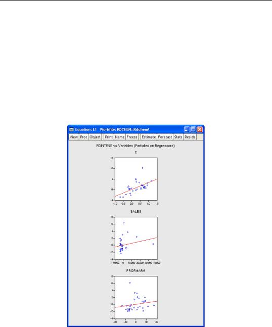
To display leverage plots in EViews select View/ Stability Diagnostics/Leverage Plots.... EViews will then display a dialog which lets you choose some simple options for the leverage plots.
The Variables to plot box lets you enter which variables, or coefficients in a non-linear equation, you wish to plot. By default this box will be filled in with the original regressors from your equation. Note that EViews will let you enter variables that were not in the original equation, in which case the plot will simply show the original equation residuals plotted against the residuals from a regression of the new variable against the original regressors.
Stability Diagnostics—183
To add a regression line to each scatter plot, select the Add fit lines checkbox. If you do not wish to create plots of the partialled variables, but would rather plot the original regression residuals against the raw regressors, unselect the Partial out variables checkbox.
Finally, if you wish to save the partial residuals for each variable into a series in the workfile, you may enter a naming suffix in the Enter a naming suffix to save the variables as a series box. EViews will then append the name of each variable to the suffix you entered as the name of the created series.
We illustrate using an example taken from Wooldridge (2000, Example 9.8) for the regression of R&D expenditures (RDINTENS) on sales (SALES), profits (PROFITMARG), and a constant (using the workfile “Rdchem.WF1”). The leverage plots for equation E1 are displayed here:
Influence Statistics
Influence statistics are a method of discovering influential observations, or outliers. They are a measure of the difference that a single observation makes to the regression results, or

184—Chapter 23. Specification and Diagnostic Tests
how different an observation is from the other observations in an equation’s sample. EViews provides a selection of six different influence statistics: RStudent, DRResid, DFFITS, CovRatio, HatMatrix and DFBETAS.
•RStudent is the studentized residual; the residual of the equation at that observation divided by an estimate of its standard deviation:
|
|
|
|
ei |
|
ei = |
|
(23.44) |
|||
---------------------------- |
|||||
|
|
|
s(i) |
1 – hi |
|
where ei is the original residual for that observation, s(i) |
is the variance of the |
||||
residuals that would have resulted had observation i not been included in the estimation, and hi is the i-th diagonal element of the Hat Matrix, i.e. xi(X'X)–1xi . The RStudent is also numerically identical to the t-statistic that would result from putting a dummy variable in the original equation which is equal to 1 on that particular observation and zero elsewhere. Thus it can be interpreted as a test for the significance of that observation.
•DFFITS is the scaled difference in fitted values for that observation between the original equation and an equation estimated without that observation, where the scaling is done by dividing the difference by an estimate of the standard deviation of the fit:
DFFITSi = |
|
|
hi |
|
1 § 2 |
|
ei |
(23.45) |
|
|
|
|
|||||
------------- |
|
---------------------------- |
||||||
|
|
1 |
– hi |
|
|
s(i) |
1 – hi |
|
|
|
|
|
|||||
•DRResid is the dropped residual, an estimate of the residual for that observation had the equation been run without that observation’s data.
•COVRATIO is the ratio of the determinant of the covariance matrix of the coefficients from the original equation to the determinant of the covariance matrix from an equation without that observation.
•HatMatrix reports the i-th diagonal element of the Hat Matrix: xi(X¢X)–1xi .
•DFBETAS are the scaled difference in the estimated betas between the original equation and an equation estimated without that observation:
DFBETASi, j |
= |
bj |
– bj(i) |
s------------(i) |
-------------------- (23.46) |
||
|
|
var(bj) |
where bj is the original equation’s coefficient estimate, and bj(i) is the coefficient estimate from an equation without observation i .
Stability Diagnostics—185
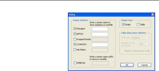
To display influence statistics in EViews select View/Stability
Diagnostics/Influence Statistics. EViews will bring up a dialog where you can choose how you wish to display the statistics. The Output statistics box lets you choose which statistics you would like to calculate, and whether to store them as a series in your workfile. Simply check the check box next to the statistics you would like to cal-
culate, and, optionally, enter the name of the series you would like to be created. Note that for the DFBETAS statistics you should enter a naming suffix, rather than the name of the series. EViews will then create the series with the name of the coefficient followed by the naming suffix you provide.
The Output type box lets you select whether to display the statistics in graph form, or in table form, or both. If both boxes are checked, EViews will create a spool object containing both tables and graphs.
If you select to display the statistics in tabular form, then a new set of options will be enabled, governing how the table is formed. By default, EViews will only display 100 rows of the statistics in the table (although note that if your equation has less than 100 observations, all of the statistics will be displayed). You can change this number by changing the Number of obs to include combo box. EViews will display the statistics sorted from highest to lowest, where the Residuals are used for the sort order. You can change which statistic is used to sort by using the Select by combo box. Finally, you can change the sort order to be by observation order rather than by one of the statistics by using the Display in observation order check box.
We illustrate using the equation E1 from the “Rdchem.WF1” workfile. A plot of the DFFITS and COVRATIOs clearly shows that observation 10 is an outlier.