136—Chapter 22. Forecasting from an Equation

By default, the combo box is set to

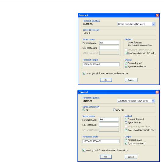
Ignore formulae within series, so that LOGHS and LOGHSLAG are viewed as ordinary series. Note that since EViews ignores the expressions underlying the auto-updating series, you may only forecast the dependent series LOGHS, and there are no dynamics implied by the equation.

Alternatively, you may instruct EViews to use the expressions in place of all auto-updating series by changing the combo box setting to

Substitute formulae within series.

If you elect to substitute the formulae, the Forecast dialog will change to reflect the use of the underlying expressions as you may now choose between forecasting HS or LOG(HS). We also see that when you use the substituted expressions you are able to perform either dynamic or static forecasting.

It is worth noting that substituting expressions yields a Forecast dialog that offers the same options as if you were to forecast from the second equation specification above—using LOG(HS) as the dependent series

expression, and LOG(HS(-1)) as an independent series expression.

Forecasting with Nonlinear and PDL Specifications

As explained above, forecast errors can arise from two sources: coefficient uncertainty and innovation uncertainty. For linear regression models, the forecast standard errors account for both coefficient and innovation uncertainty. However, if the model is specified by expression (or if it contains a PDL specification), then the standard errors ignore coefficient uncertainty. EViews will display a message in the status line at the bottom of the EViews window when forecast standard errors only account for innovation uncertainty.

References

Pindyck, Robert S. and Daniel L. Rubinfeld (1998). Econometric Models and Economic Forecasts, 4th edition, New York: McGraw-Hill.