Forecasts with Lagged Dependent Variables—123

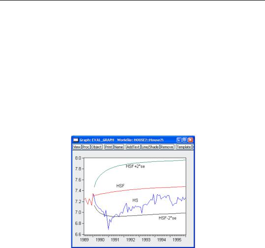
For the example output, the bias proportion is large, indicating that the mean of the forecasts does a poor job of tracking the mean of the dependent variable. To check this, we will plot the forecasted series together with the actual series in the forecast sample with the two standard error bounds. Suppose we saved the forecasts and their standard errors as HSF and HSFSE, respectively. Then the plus and minus two standard error series can be generated by the commands:

smpl 1990m02 1996m01

series hsf_high = hsf + 2*hsfse series hsf_low = hsf - 2*hsfse

Create a group containing the four series. You can highlight the four series HS, HSF, HSF_HIGH, and HSF_LOW, double click on the selected area, and select Open Group, or you can select Quick/Show… and enter the four series names. Once you have the group open, select View/Graph... and select Line & Symbol from the left side of the dialog.

The forecasts completely miss the downturn at the start of the 1990’s, but, subsequent to the recovery, track the trend reasonably well from 1992 to 1996.

Forecasts with Lagged Dependent Variables

Forecasting is complicated by the presence of lagged dependent variables on the right-hand side of the equation. For example, we can augment the earlier specification to include the first lag of Y:

y c x z y(-1)

and click on the Forecast button and fill out the series names in the dialog as above. There is some question, however, as to how we should evaluate the lagged value of Y that appears

124—Chapter 22. Forecasting from an Equation

on the right-hand side of the equation. There are two possibilities: dynamic forecasting and static forecasting.

Dynamic Forecasting

If you select dynamic forecasting, EViews will perform a multi-step forecast of Y, beginning at the start of the forecast sample. For our single lag specification above:

•The initial observation in the forecast sample will use the actual value of lagged Y. Thus, if S is the first observation in the forecast sample, EViews will compute:

where yS – 1 is the value of the lagged endogenous variable in the period prior to the start of the forecast sample. This is the one-step ahead forecast.

• Forecasts for subsequent observations will use the previously forecasted values of Y:

• These forecasts may differ significantly from the one-step ahead forecasts.

If there are additional lags of Y in the estimating equation, the above algorithm is modified to account for the non-availability of lagged forecasted values in the additional period. For example, if there are three lags of Y in the equation:

•The first observation (S ) uses the actual values for all three lags, yS – 3 , yS – 2 , and yS – 1 .

•The second observation (S + 1 ) uses actual values for yS – 2 and, yS – 1 and the fore-

casted value yˆ S of the first lag of yS + 1 .

• The third observation (S + 2 ) will use the actual values for yS – 1 , and forecasted values yˆ S + 1 and yˆ S for the first and second lags of yS + 2 .

• All subsequent observations will use the forecasted values for all three lags.

The selection of the start of the forecast sample is very important for dynamic forecasting. The dynamic forecasts are true multi-step forecasts (from the start of the forecast sample), since they use the recursively computed forecast of the lagged value of the dependent variable. These forecasts may be interpreted as the forecasts for subsequent periods that would be computed using information available at the start of the forecast sample.

Dynamic forecasting requires that data for the exogenous variables be available for every observation in the forecast sample, and that values for any lagged dependent variables be observed at the start of the forecast sample (in our example, yS – 1 , but more generally, any lags of y ). If necessary, the forecast sample will be adjusted.

126—Chapter 22. Forecasting from an Equation

Forecasting with AR Errors

For equations with AR errors, EViews adds forecasts of the residuals from the equation to the forecast of the structural model that is based on the right-hand side variables.

In order to compute an estimate of the residual, EViews requires estimates or actual values of the lagged residuals. For the first observation in the forecast sample, EViews will use presample data to compute the lagged residuals. If the pre-sample data needed to compute the lagged residuals are not available, EViews will adjust the forecast sample, and backfill the forecast series with actual values (see the discussion of “Adjustment for Missing Values” on page 118).

If you choose the Dynamic option, both the lagged dependent variable and the lagged residuals will be forecasted dynamically. If you select Static, both will be set to the actual lagged values. For example, consider the following AR(2) model:

sequent observations, the dynamic forecast will always use the residuals based upon the multi-step forecasts, while the static forecast will use the one-step ahead forecast residuals.

Forecasting with MA Errors

In general, you need not concern yourselves with the details of MA forecasting, since EViews will do all of the work for you. However, for those of you who are interested in the details of dynamic forecasting, the following discussion should aid you in relating EViews results with those obtained from other sources.

We begin by noting that the key step in computing forecasts using MA terms is to obtain fitted values for the innovations in the pre-forecast sample period. For example, if you are performing dynamic forecasting of the values of y , beginning in period S , with a simple

MA(q ) process:

you will need values for the pre-forecast sample innovations, eS – 1, eS – 2, º, eS – q . Similarly, constructing a static forecast for a given period will require estimates of the q lagged innovations at every period in the forecast sample.

If your equation is estimated with backcasting turned on, EViews will perform backcasting to obtain these values. If your equation is estimated with backcasting turned off, or if the forecast sample precedes the estimation sample, the initial values will be set to zero.

Backcast Sample

The first step in obtaining pre-forecast innovations is obtaining estimates of the pre-estima- tion sample innovations: e0, e–1, e–2, º, e–q . (For notational convenience, we normalize the start and end of the estimation sample to t = 1 and t = T , respectively.)

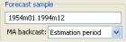
EViews offers two different approaches for obtaining esti- mates—you may use the MA backcast combo box to choose between the default Estimation period and the Forecast available (v5) methods.

The Estimation period method uses data for the estimation sample to compute backcast estimates. Then as in estimation (“Backcasting MA terms” on page 102), the q values for the innovations beyond the estimation sample are set to zero:

EViews then uses the unconditional residuals to perform the backward recursion:

for t = T, º, 0, º, –(q – 1) to obtain the pre-estimation sample residuals. Note that absent changes in the data, using Estimation period produces pre-forecast sample innovations that match those employed in estimation (where applicable).

The Forecast available (v5) method offers different approaches for dynamic and static forecasting:

•For dynamic forecasting, EViews applies the backcasting procedure using data from the beginning of the estimation sample to either the beginning of the forecast period, or the end of the estimation sample, whichever comes first.

•For static forecasting, the backcasting procedure uses data from the beginning of the estimation sample to the end of the forecast period.

For both dynamic and static forecasts, the post-backcast sample innovations are initialized to zero and the backward recursion is employed to obtain estimates of the pre-estimation

128—Chapter 22. Forecasting from an Equation

sample innovations. Note that Forecast available (v5) does not guarantee that the pre-sam- ple forecast innovations match those employed in estimation.

Pre-Forecast Innovations

Given the backcast estimates of the pre-estimation sample residuals, forward recursion is used to obtain values for the pre-forecast sample innovations.

For dynamic forecasting, one need only obtain innovation values for the q periods prior to the start of the forecast sample; all subsequent innovations are set to zero. EViews obtains

for t = 1, º, S – 1 , where S is the beginning of the forecast period

Static forecasts perform the forward recursion through the end of the forecast sample so that innovations are estimated through the last forecast period. Computation of the static forecast for each period uses the q lagged estimated innovations. Extending the recursion produces a series of one-step ahead forecasts of both the structural model and the innovations.

Additional Notes

Note that EViews computes the residuals used in backcast and forward recursion from the observed data and estimated coefficients. If EViews is unable to compute values for the unconditional residuals ut for a given period, the sequence of innovations and forecasts will be filled with NAs. In particular, static forecasts must have valid data for both the dependent and explanatory variables for all periods from the beginning of estimation sample to the end of the forecast sample, otherwise the backcast values of the innovations, and hence the forecasts will contain NAs. Likewise, dynamic forecasts must have valid data from the beginning of the estimation period through the start of the forecast period.

Example

As an example of forecasting from ARMA models, consider forecasting the monthly new housing starts (HS) series. The estimation period is 1959M01–1984M12 and we forecast for the period 1985M01–1991M12. We estimated the following simple multiplicative seasonal autoregressive model,

hs c ar(1) sar(12)

yielding: