


Chapter 22. Forecasting from an Equation
This chapter describes procedures for forecasting and computing fitted values from a single equation. The techniques described here are for forecasting with equation objects estimated using regression methods. Forecasts from equations estimated by specialized techniques, such as ARCH, binary, ordered, tobit, and count methods, are discussed in the corresponding chapters. Forecasting from a series using exponential smoothing methods is explained in “Exponential Smoothing” on page 364 of User’s Guide I, and forecasting using multiple equations and models is described in Chapter 34. “Models,” on page 511.
Forecasting from Equations in EViews
To illustrate the process of forecasting from an estimated equation, we begin with a simple example. Suppose we have data on the logarithm of monthly housing starts (HS) and the logarithm of the S&P index (SP) over the period 1959M01–1996M0. The data are contained in the workfile “House1.WF1” which contains observations for 1959M01–1998M12 so that we may perform out-of-sample forecasts.
We estimate a regression of HS on a constant, SP, and the lag of HS, with an AR(1) to correct for residual serial correlation, using data for the period 1959M01–1990M01, and then use the model to forecast housing starts under a variety of settings. Following estimation, the equation results are held in the equation object EQ01:
Dependent Variable: HS
Method: Least Squares
Date: 08/09/09 Time: 07:45
Sample (adjusted): 1959M03 1990M01
Included observations: 371 after adjustments
Convergence achieved after 6 iterations
Variable |
Coefficient |
Std. Error |
t-Statistic |
Prob. |
|
|
|
|
|
C |
0.321924 |
0.117278 |
2.744973 |
0.0063 |
HS(-1) |
0.952653 |
0.016218 |
58.74151 |
0.0000 |
SP |
0.005222 |
0.007588 |
0.688248 |
0.4917 |
AR(1) |
-0.271254 |
0.052114 |
-5.205025 |
0.0000 |
|
|
|
|
|
|
|
|
|
|
R-squared |
0.861373 |
Mean dependent var |
7.324051 |
|
Adjusted R-squared |
0.860240 |
S.D. dependent var |
0.220996 |
|
S.E. of regression |
0.082618 |
Akaike info criterion |
-2.138453 |
|
Sum squared resid |
2.505050 |
Schwarz criterion |
-2.096230 |
|
Log likelihood |
400.6830 |
Hannan-Quinn criter. |
-2.121683 |
|
F-statistic |
760.1338 |
Durbin-W atson stat |
2.013460 |
|
Prob(F-statistic) |
0.000000 |
|
|
|
|
|
|
|
|
|
|
|
|
|
Inverted AR Roots |
-.27 |
|
|
|
|
|
|
|
|
|
|
|
|
|
112—Chapter 22. Forecasting from an Equation
Note that the estimation sample is adjusted by two observations to account for the first difference of the lagged endogenous variable used in deriving AR(1) estimates for this model.
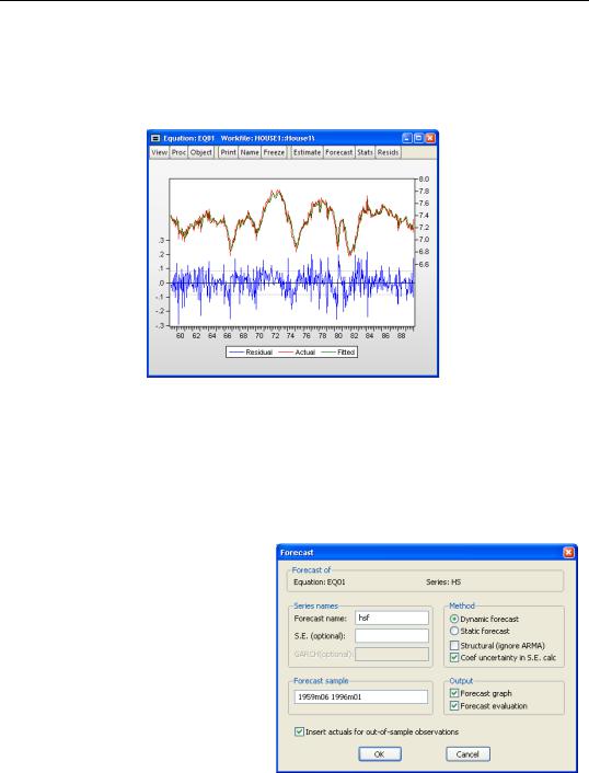
To get a feel for the fit of the model, select View/Actual, Fitted, Residual…, then choose
Actual, Fitted, Residual Graph:
The actual and fitted values depicted on the upper portion of the graph are virtually indistinguishable. This view provides little control over the process of producing fitted values, and does not allow you to save your fitted values. These limitations are overcome by using EViews built-in forecasting procedures to compute fitted values for the dependent variable.
How to Perform a Forecast
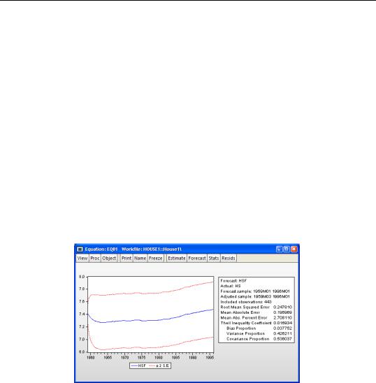
To forecast HS from this equation, push the Forecast button on the equation toolbar, or select Proc/Forecast….
At the top of the Forecast dialog, EViews displays information about the forecast. Here, we show a basic version of the dialog showing that we are forecasting values for the dependent series HS using the estimated EQ01. More complex settings are described in “Forecasting from Equations with Expressions” on page 130.
You should provide the following information:

Forecasting from Equations in EViews—113
•Forecast name. Fill in the edit box with the series name to be given to your forecast. EViews suggests a name, but you can change it to any valid series name. The name should be different from the name of the dependent variable, since the forecast procedure will overwrite data in the specified series.
•S.E. (optional). If desired, you may provide a name for the series to be filled with the forecast standard errors. If you do not provide a name, no forecast errors will be saved.
•GARCH (optional). For models estimated by ARCH, you will be given a further option of saving forecasts of the conditional variances (GARCH terms). See Chapter 24. “ARCH and GARCH Estimation,” on page 195 for a discussion of GARCH estimation.
•Forecasting method. You have a choice between Dynamic and Static forecast methods. Dynamic calculates dynamic, multi-step forecasts starting from the first period in the forecast sample. In dynamic forecasting, previously forecasted values for the lagged dependent variables are used in forming forecasts of the current value (see “Forecasts with Lagged Dependent Variables” on page 123 and “Forecasting with ARMA Errors” on page 125). This choice will only be available when the estimated equation contains dynamic components, e.g., lagged dependent variables or ARMA terms. Static calculates a sequence of one-step ahead forecasts, using the actual, rather than forecasted values for lagged dependent variables, if available.
You may elect to always ignore coefficient uncertainty in computing forecast standard errors (when relevant) by unselecting the Coef uncertainty in S.E. calc box.
In addition, in specifications that contain ARMA terms, you can set the Structural option, instructing EViews to ignore any ARMA terms in the equation when forecasting. By default, when your equation has ARMA terms, both dynamic and static solution methods form forecasts of the residuals. If you select Structural, all forecasts will ignore the forecasted residuals and will form predictions using only the structural part of the ARMA specification.
•Sample range. You must specify the sample to be used for the forecast. By default, EViews sets this sample to be the workfile sample. By specifying a sample outside the sample used in estimating your equation (the estimation sample), you can instruct EViews to produce out-of-sample forecasts.
Note that you are responsible for supplying the values for the independent variables in the out-of-sample forecasting period. For static forecasts, you must also supply the values for any lagged dependent variables.
•Output. You can choose to see the forecast output as a graph or a numerical forecast evaluation, or both. Forecast evaluation is only available if the forecast sample includes observations for which the dependent variable is observed.
114—Chapter 22. Forecasting from an Equation
•Insert actuals for out-of-sample observations. By default, EViews will fill the forecast series with the values of the actual dependent variable for observations not in the forecast sample. This feature is convenient if you wish to show the divergence of the forecast from the actual values; for observations prior to the beginning of the forecast sample, the two series will contain the same values, then they will diverge as the forecast differs from the actuals. In some contexts, however, you may wish to have forecasted values only for the observations in the forecast sample. If you uncheck this option, EViews will fill the out-of-sample observations with missing values.
Note that when performing forecasts from equations specified using expressions or autoupdating series, you may encounter a version of the Forecast dialog that differs from the basic dialog depicted above. See “Forecasting from Equations with Expressions” on page 130 for details.
An Illustration
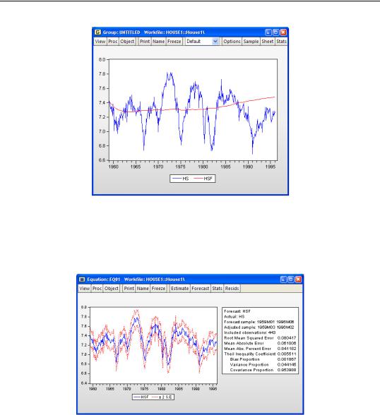
Suppose we produce a dynamic forecast using EQ01 over the sample 1959M01 to 1996M01. The forecast values will be placed in the series HSF, and EViews will display a graph of the forecasts and the plus and minus two standard error bands, as well as a forecast evaluation:
This is a dynamic forecast for the period from 1959M01 through 1996M01. For every period, the previously forecasted values for HS(-1) are used in forming a forecast of the subsequent value of HS. As noted in the output, the forecast values are saved in the series HSF. Since HSF is a standard EViews series, you may examine your forecasts using all of the standard tools for working with series objects.
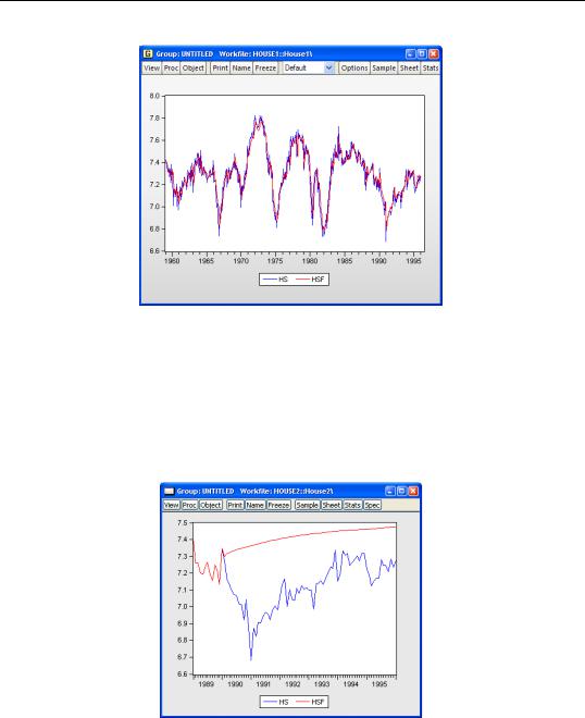
For example, we may examine the actual versus fitted values by creating a group containing HS and HSF, and plotting the two series. Select HS and HSF in the workfile window, then right-mouse click and select Open/as Group. Then select View/Graph... and select Line & Symbol in the Graph Type/Basic type page to display a graph of the two series:
An Illustration—115
Note the considerable difference between this actual and fitted graph and the Actual, Fitted, Residual Graph depicted above.
To perform a series of one-step ahead forecasts, click on Forecast on the equation toolbar, and select Static forecast. Make certain that the forecast sample is set to “1959m01 1995m06”. Click on OK. EViews will display the forecast results:
We may also compare the actual and fitted values from the static forecast by examining a line graph of a group containing HS and the new HSF.
116—Chapter 22. Forecasting from an Equation
The one-step ahead static forecasts are more accurate than the dynamic forecasts since, for each period, the actual value of HS(-1) is used in forming the forecast of HS. These one-step ahead static forecasts are the same forecasts used in the Actual, Fitted, Residual Graph displayed above.
Lastly, we construct a dynamic forecast beginning in 1990M02 (the first period following the estimation sample) and ending in 1996M01. Keep in mind that data are available for SP for this entire period. The plot of the actual and the forecast values for 1989M01 to 1996M01 is given by:
Since we use the default settings for out-of-forecast sample values, EViews backfills the forecast series prior to the forecast sample (up through 1990M01), then dynamically forecasts HS for each subsequent period through 1996M01. This is the forecast that you would have