
- •Preface
- •Part IV. Basic Single Equation Analysis
- •Chapter 18. Basic Regression Analysis
- •Equation Objects
- •Specifying an Equation in EViews
- •Estimating an Equation in EViews
- •Equation Output
- •Working with Equations
- •Estimation Problems
- •References
- •Chapter 19. Additional Regression Tools
- •Special Equation Expressions
- •Robust Standard Errors
- •Weighted Least Squares
- •Nonlinear Least Squares
- •Stepwise Least Squares Regression
- •References
- •Chapter 20. Instrumental Variables and GMM
- •Background
- •Two-stage Least Squares
- •Nonlinear Two-stage Least Squares
- •Limited Information Maximum Likelihood and K-Class Estimation
- •Generalized Method of Moments
- •IV Diagnostics and Tests
- •References
- •Chapter 21. Time Series Regression
- •Serial Correlation Theory
- •Testing for Serial Correlation
- •Estimating AR Models
- •ARIMA Theory
- •Estimating ARIMA Models
- •ARMA Equation Diagnostics
- •References
- •Chapter 22. Forecasting from an Equation
- •Forecasting from Equations in EViews
- •An Illustration
- •Forecast Basics
- •Forecasts with Lagged Dependent Variables
- •Forecasting with ARMA Errors
- •Forecasting from Equations with Expressions
- •Forecasting with Nonlinear and PDL Specifications
- •References
- •Chapter 23. Specification and Diagnostic Tests
- •Background
- •Coefficient Diagnostics
- •Residual Diagnostics
- •Stability Diagnostics
- •Applications
- •References
- •Part V. Advanced Single Equation Analysis
- •Chapter 24. ARCH and GARCH Estimation
- •Basic ARCH Specifications
- •Estimating ARCH Models in EViews
- •Working with ARCH Models
- •Additional ARCH Models
- •Examples
- •References
- •Chapter 25. Cointegrating Regression
- •Background
- •Estimating a Cointegrating Regression
- •Testing for Cointegration
- •Working with an Equation
- •References
- •Binary Dependent Variable Models
- •Ordered Dependent Variable Models
- •Censored Regression Models
- •Truncated Regression Models
- •Count Models
- •Technical Notes
- •References
- •Chapter 27. Generalized Linear Models
- •Overview
- •How to Estimate a GLM in EViews
- •Examples
- •Working with a GLM Equation
- •Technical Details
- •References
- •Chapter 28. Quantile Regression
- •Estimating Quantile Regression in EViews
- •Views and Procedures
- •Background
- •References
- •Chapter 29. The Log Likelihood (LogL) Object
- •Overview
- •Specification
- •Estimation
- •LogL Views
- •LogL Procs
- •Troubleshooting
- •Limitations
- •Examples
- •References
- •Part VI. Advanced Univariate Analysis
- •Chapter 30. Univariate Time Series Analysis
- •Unit Root Testing
- •Panel Unit Root Test
- •Variance Ratio Test
- •BDS Independence Test
- •References
- •Part VII. Multiple Equation Analysis
- •Chapter 31. System Estimation
- •Background
- •System Estimation Methods
- •How to Create and Specify a System
- •Working With Systems
- •Technical Discussion
- •References
- •Vector Autoregressions (VARs)
- •Estimating a VAR in EViews
- •VAR Estimation Output
- •Views and Procs of a VAR
- •Structural (Identified) VARs
- •Vector Error Correction (VEC) Models
- •A Note on Version Compatibility
- •References
- •Chapter 33. State Space Models and the Kalman Filter
- •Background
- •Specifying a State Space Model in EViews
- •Working with the State Space
- •Converting from Version 3 Sspace
- •Technical Discussion
- •References
- •Chapter 34. Models
- •Overview
- •An Example Model
- •Building a Model
- •Working with the Model Structure
- •Specifying Scenarios
- •Using Add Factors
- •Solving the Model
- •Working with the Model Data
- •References
- •Part VIII. Panel and Pooled Data
- •Chapter 35. Pooled Time Series, Cross-Section Data
- •The Pool Workfile
- •The Pool Object
- •Pooled Data
- •Setting up a Pool Workfile
- •Working with Pooled Data
- •Pooled Estimation
- •References
- •Chapter 36. Working with Panel Data
- •Structuring a Panel Workfile
- •Panel Workfile Display
- •Panel Workfile Information
- •Working with Panel Data
- •Basic Panel Analysis
- •References
- •Chapter 37. Panel Estimation
- •Estimating a Panel Equation
- •Panel Estimation Examples
- •Panel Equation Testing
- •Estimation Background
- •References
- •Part IX. Advanced Multivariate Analysis
- •Chapter 38. Cointegration Testing
- •Johansen Cointegration Test
- •Single-Equation Cointegration Tests
- •Panel Cointegration Testing
- •References
- •Chapter 39. Factor Analysis
- •Creating a Factor Object
- •Rotating Factors
- •Estimating Scores
- •Factor Views
- •Factor Procedures
- •Factor Data Members
- •An Example
- •Background
- •References
- •Appendix B. Estimation and Solution Options
- •Setting Estimation Options
- •Optimization Algorithms
- •Nonlinear Equation Solution Methods
- •References
- •Appendix C. Gradients and Derivatives
- •Gradients
- •Derivatives
- •References
- •Appendix D. Information Criteria
- •Definitions
- •Using Information Criteria as a Guide to Model Selection
- •References
- •Appendix E. Long-run Covariance Estimation
- •Technical Discussion
- •Kernel Function Properties
- •References
- •Index
- •Symbols
- •Numerics

104—Chapter 21. Time Series Regression
terms in your model, you lose degrees of freedom, and may sacrifice stability and reliability of your estimates.
If the underlying roots of the MA process have modulus close to one, you may encounter estimation difficulties, with EViews reporting that it cannot improve the sum-of-squares or that it failed to converge in the maximum number of iterations. This behavior may be a sign that you have over-differenced the data. You should check the correlogram of the series to determine whether you can re-estimate with one less round of differencing.
Lastly, if you continue to have problems, you may wish to turn off MA backcasting.
TSLS with ARIMA errors
Two-stage least squares or instrumental variable estimation with ARIMA errors pose no particular difficulties.
For a discussion of how to estimate TSLS specifications with ARMA errors, see “Nonlinear Two-stage Least Squares” on page 62.
Nonlinear Models with ARMA errors
EViews will estimate nonlinear ordinary and two-stage least squares models with autoregressive error terms. For details, see the discussion in “Nonlinear Least Squares,” beginning on page 40.
Weighted Models with ARMA errors
EViews does not offer built-in procedures to automatically estimate weighted models with ARMA error terms—if you add AR terms to a weighted model, the weighting series will be ignored. You can, of course, always construct the weighted series and then perform estimation using the weighted data and ARMA terms. Note that this procedure implies a very specific assumption about the properties of your data.
ARMA Equation Diagnostics
ARMA Structure
This set of views provides access to several diagnostic views that help you assess the structure of the ARMA portion of the estimated equation. The view is currently available only for models specified by list that includes at least one AR or MA term and estimated by least squares. There are three views available: roots, correlogram, and impulse response.
ARMA Equation Diagnostics—105
To display the ARMA structure, select View/ ARMA Structure... from the menu of an estimated equation. If the equation type supports this view and there are no ARMA components in the specification, EViews will open the ARMA Diagnostic Views dialog:
On the left-hand side of the dialog, you will select one of the three types of diagnostics. When you click on one of the types, the
right-hand side of the dialog will change to show you the options for each type.
Roots
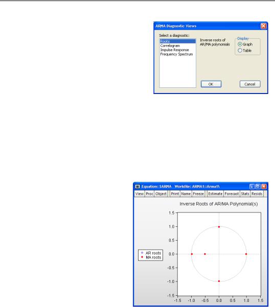
The roots view displays the inverse roots of the AR and/or MA characteristic polynomial. The roots may be displayed as a graph or as a table by selecting the appropriate radio button.
The graph view plots the roots in the complex plane where the horizontal axis is the real part and the vertical axis is the imaginary part of each root.
If the estimated ARMA process is (covariance) stationary, then all AR roots should lie inside the unit circle. If the estimated ARMA process is invertible, then all MA roots should lie inside the unit circle. The table view displays all roots in order of decreasing modulus (square root of the sum of squares of the real and imaginary parts).
For imaginary roots (which come in conjugate pairs), we also display the cycle corresponding to that root. The
cycle is computed as 2p § a , where a = atan(i § r), and i and r are
the imaginary and real parts of the root, respectively. The cycle for a real root is infinite and is not reported.
106—Chapter 21. Time Series Regression
Inverse Roots of AR/MA Polynomial(s)
Specification: R C AR(1) SAR(4) MA(1) SMA(4)
Date: 08/09/09 Time: 07:22
Sample: 1954M01 1994M12
Included observations: 470
|
AR Root(s) |
Modulus |
Cycle |
|
|
|
|
|
|
|
|
4. |
16e-17 ± 0.985147i |
0.985147 |
4.000000 |
-0.985147 |
0.985147 |
|
|
0. |
985147 |
0.985147 |
|
0. |
983011 |
0.983011 |
|
|
|
||
No root lies outside the unit circle. |
|
||
ARMA model is stationary. |
|
|
|
|
|
|
|
|
|
|
|
|
MA Root(s) |
Modulus |
Cycle |
|
|
|
|
|
|
|
|
-0.989949 |
0.989949 |
|
|
-2.36e-16 ± 0.989949i |
0.989949 |
4.000000 |
|
0. |
989949 |
0.989949 |
|
-0.513572 |
0.513572 |
|
|
No root lies outside the unit circle.
ARMA model is invertible.
Correlogram
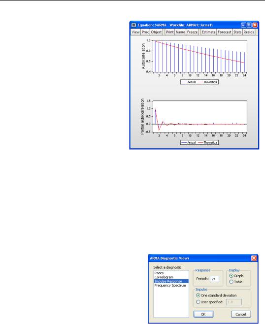
The correlogram view compares the autocorrelation pattern of the structural residuals and that of the estimated model for a specified number of periods (recall that the structural residuals are the residuals after removing the effect of the fitted exogenous regressors but not the ARMA terms). For a properly specified model, the residual and theoretical (estimated) autocorrelations and partial autocorrelations should be “close”.
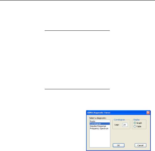
To perform the comparison, simply select the Correlogram diagnostic, specify a number of lags to be evaluated, and a display format (Graph or Table).
ARMA Equation Diagnostics—107
Here, we have specified a graphical comparison over 24 periods/lags. The graph view plots the autocorrelations and partial autocorrelations of the sample structural residuals and those that are implied from the estimated ARMA parameters. If the estimated ARMA model is not stationary, only the sample second moments from the structural residuals are plotted.
The table view displays the numerical values for each of the second moments and the difference between from the estimated theoretical. If the estimated ARMA model is not stationary, the theoretical second moments
implied from the estimated ARMA parameters will be filled with NAs.
Note that the table view starts from lag zero, while the graph view starts from lag one.
Impulse Response
The ARMA impulse response view traces the response of the ARMA part of the estimated equation to shocks in the innovation.
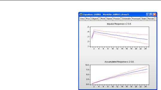
An impulse response function traces the response to a one-time shock in the innovation. The accumulated response is the accumulated sum of the impulse responses. It can be interpreted as the response to step impulse where the same shock occurs in every period from the first.
To compute the impulse response (and accumulated responses), select the Impulse Response diagnostic, enter the number of periods, and display type, and define the shock. For the latter, you have the choice of using a one standard deviation shock (using the standard error of the regression for the estimated equation), or providing a user specified value. Note that if you select a one standard deviation shock, EViews will take
account of innovation uncertainty when estimating the standard errors of the responses.
108—Chapter 21. Time Series Regression
If the estimated ARMA model is stationary, the impulse responses will asymptote to zero, while the accumulated responses will asymptote to its long-run value. These asymptotic values will be shown as dotted horizontal lines in the graph view.
For a highly persistent near unit root but stationary process, the asymptotes may not be drawn in the graph for a short horizon. For a table view, the asymptotic values (together with its standard errors) will be shown at the bottom of the table. If the estimated ARMA process is not stationary, the asymptotic values will not be displayed since they do not exist.
ARMA Frequency Spectrum
The ARMA frequency spectrum view of an ARMA equation shows the spectrum of the estimated ARMA terms in the frequency domain, rather than the typical time domain. Whereas viewing the ARMA terms in the time domain lets you view the autocorrelation functions of the data, viewing them in the frequency domain lets you observe more complicated cyclical characteristics.
The spectrum of an ARMA process can be written as a function of its frequency, l , where l is measured in radians, and thus takes values from –p to p . However since the spectrum is symmetric around 0, it is EViews displays it in the range [0, p].
To show the frequency spectrum, select View/ARMA Structure... from the equation toolbar, choose Frequency spectrum from the Select a diagnostic list box, and then select a display format (Graph or Table).
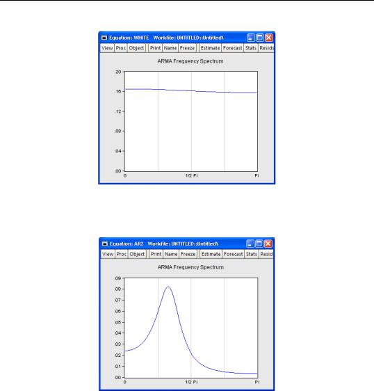
If a series is white noise, the frequency spectrum should be flat, that is a horizontal line. Here we display the graph of a series generated as random normals, and indeed, the graph is approximately a flat line.
ARMA Equation Diagnostics—109
If a series has strong AR components, the shape of the frequency spectrum will contain peaks at points of high cyclical frequencies. Here we show a typical AR(2) model, where the data were generated such that r1 = 0.7 and r2 = –0.5 .
Q-statistics
If your ARMA model is correctly specified, the residuals from the model should be nearly white noise. This means that there should be no serial correlation left in the residuals. The Durbin-Watson statistic reported in the regression output is a test for AR(1) in the absence of lagged dependent variables on the right-hand side. As discussed in “Correlograms and Q- statistics” on page 87, more general tests for serial correlation in the residuals may be carried out with View/Residual Diagnostics/Correlogram-Q-statistic and View/Residual Diagnostics/Serial Correlation LM Test….
