ARIMA Theory

94—Chapter 21. Time Series Regression

The autoregressive and moving average specifications can be combined to form an ARMA(p, q ) specification:

Although econometricians typically use ARIMA models applied to the residuals from a regression model, the specification can also be applied directly to a series. This latter approach provides a univariate model, specifying the conditional mean of the series as a constant, and measuring the residuals as differences of the series from its mean.

Principles of ARIMA Modeling (Box-Jenkins 1976)

In ARIMA forecasting, you assemble a complete forecasting model by using combinations of the three building blocks described above. The first step in forming an ARIMA model for a series of residuals is to look at its autocorrelation properties. You can use the correlogram view of a series for this purpose, as outlined in “Correlogram” on page 333 of User’s Guide I.

This phase of the ARIMA modeling procedure is called identification (not to be confused with the same term used in the simultaneous equations literature). The nature of the correlation between current values of residuals and their past values provides guidance in selecting an ARIMA specification.

The autocorrelations are easy to interpret—each one is the correlation coefficient of the current value of the series with the series lagged a certain number of periods. The partial autocorrelations are a bit more complicated; they measure the correlation of the current and lagged series after taking into account the predictive power of all the values of the series with smaller lags. The partial autocorrelation for lag 6, for example, measures the added predictive power of ut – 6 when u1, º, ut – 5 are already in the prediction model. In fact, the partial autocorrelation is precisely the regression coefficient of ut – 6 in a regression where the earlier lags are also used as predictors of ut .

If you suspect that there is a distributed lag relationship between your dependent (left-hand) variable and some other predictor, you may want to look at their cross correlations before carrying out estimation.

The next step is to decide what kind of ARIMA model to use. If the autocorrelation function dies off smoothly at a geometric rate, and the partial autocorrelations were zero after one lag, then a first-order autoregressive model is appropriate. Alternatively, if the autocorrelations were zero after one lag and the partial autocorrelations declined geometrically, a firstorder moving average process would seem appropriate. If the autocorrelations appear to have a seasonal pattern, this would suggest the presence of a seasonal ARMA structure (see “Seasonal ARMA Terms” on page 97).

For example, we can examine the correlogram of the DRI Basics housing series in the “Hs.WF1” workfile by setting the sample to “1959m01 1984m12” then selecting View/Cor-

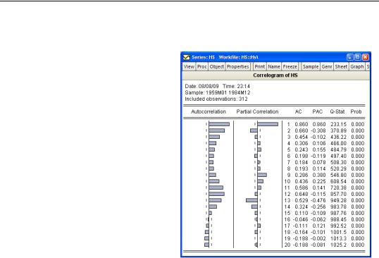
Estimating ARIMA Models—95

relogram… from the HS series toolbar. Click on OK to accept the default settings and display the result.

The “wavy” cyclical correlogram with a seasonal frequency suggests fitting a seasonal ARMA model to HS.

The goal of ARIMA analysis is a parsimonious representation of the process governing the residual. You should use only enough AR and MA terms to fit the properties of the residuals. The Akaike information criterion and Schwarz criterion provided with each set of estimates may also be used as a guide for the appropriate lag order selection.

After fitting a candidate ARIMA specification, you should verify that there are no remaining autocorrelations

that your model has not accounted for. Examine the autocorrelations and the partial autocorrelations of the innovations (the residuals from the ARIMA model) to see if any important forecasting power has been overlooked. EViews provides views for diagnostic checks after estimation.

Estimating ARIMA Models

EViews estimates general ARIMA specifications that allow for right-hand side explanatory variables. Despite the fact that these models are sometimes termed ARIMAX specifications, we will refer to this general class of models as ARIMA.

To specify your ARIMA model, you will:

•Difference your dependent variable, if necessary, to account for the order of integration.

•Describe your structural regression model (dependent variables and regressors) and add any AR or MA terms, as described above.

Differencing

The d operator can be used to specify differences of series. To specify first differencing, simply include the series name in parentheses after d. For example, d(gdp) specifies the first difference of GDP, or GDP–GDP(–1).

96—Chapter 21. Time Series Regression

More complicated forms of differencing may be specified with two optional parameters, n and s . d(x,n) specifies the n -th order difference of the series X:

where L is the lag operator. For example, d(gdp,2) specifies the second order difference of GDP:

d(gdp,2) = gdp – 2*gdp(–1) + gdp(–2)

d(x,n,s) specifies n -th order ordinary differencing of X with a seasonal difference at lag s :

For example, d(gdp,0,4) specifies zero ordinary differencing with a seasonal difference at lag 4, or GDP–GDP(–4).

If you need to work in logs, you can also use the dlog operator, which returns differences in the log values. For example, dlog(gdp) specifies the first difference of log(GDP) or log(GDP)–log(GDP(–1)). You may also specify the n and s options as described for the simple d operator, dlog(x,n,s).

There are two ways to estimate integrated models in EViews. First, you may generate a new series containing the differenced data, and then estimate an ARMA model using the new data. For example, to estimate a Box-Jenkins ARIMA(1, 1, 1) model for M1, you can enter:

series dm1 = d(m1)

equation eq1.ls dm1 c ar(1) ma(1)

Alternatively, you may include the difference operator d directly in the estimation specification. For example, the same ARIMA(1,1,1) model can be estimated using the command:

equation eq1.ls d(m1) c ar(1) ma(1)

The latter method should generally be preferred for an important reason. If you define a new variable, such as DM1 above, and use it in your estimation procedure, then when you forecast from the estimated model, EViews will make forecasts of the dependent variable DM1. That is, you will get a forecast of the differenced series. If you are really interested in forecasts of the level variable, in this case M1, you will have to manually transform the forecasted value and adjust the computed standard errors accordingly. Moreover, if any other transformation or lags of M1 are included as regressors, EViews will not know that they are related to DM1. If, however, you specify the model using the difference operator expression for the dependent variable, d(m1), the forecasting procedure will provide you with the option of forecasting the level variable, in this case M1.

The difference operator may also be used in specifying exogenous variables and can be used in equations without ARMA terms. Simply include them in the list of regressors in addition to the endogenous variables. For example:

98—Chapter 21. Time Series Regression

You can estimate this process by including ar(1) and ar(2) terms in the list of regressors. With quarterly data, you might want to add a sar(4) expression to take account of seasonality. If you specify the equation as,

sales c inc ar(1) ar(2) sar(4)

The parameter v is associated with the seasonal part of the process. Note that this is an AR(6) process with nonlinear restrictions on the coefficients.

You may estimate this second-order process by including both the MA(1) and MA(2) terms in your equation specification.

With quarterly data, you might want to add sma(4) to take account of seasonality. If you specify the equation as,

cs c ad ma(1) ma(2) sma(4)

then the estimated model is:

100—Chapter 21. Time Series Regression

Dependent Variable: R

Method: Least Squares

Date: 08/08/09 Time: 23:19

Sample (adjusted): 1954M06 1993M07

Included observations: 470 after adjustments

Convergence achieved after 23 iterations

MA Backcast: 1954M01 1954M05

This estimation result corresponds to the following specification,

or equivalently, to:

Note that the signs of the MA terms may be reversed from those in textbooks. Note also that the inverted roots have moduli very close to one, which is typical for many macro time series models.

Estimation Options

ARMA estimation employs the same nonlinear estimation techniques described earlier for AR estimation. These nonlinear estimation techniques are discussed further in Chapter 19. “Additional Regression Tools,” on page 41.

You may use the Options tab to control the iterative process. EViews provides a number of options that allow you to control the iterative procedure of the estimation algorithm. In general, you can rely on the EViews choices, but on occasion you may wish to override the default settings.

102—Chapter 21. Time Series Regression

To properly set starting values, you will need a little more information about how EViews assigns coefficients for the ARMA terms. As with other estimation methods, when you specify your equation as a list of variables, EViews uses the built-in C coefficient vector. It assigns coefficient numbers to the variables in the following order:

•First are the coefficients of the variables, in order of entry.

•Next come the AR terms in the order you typed them.

•The SAR, MA, and SMA coefficients follow, in that order.

Thus the following two specifications will have their coefficients in the same order:

y c x ma(2) ma(1) sma(4) ar(1) y sma(4)c ar(1) ma(2) x ma(1)

You may also assign values in the C vector using the param command:

param c(1) 50 c(2) .8 c(3) .2 c(4) .6 c(5) .1 c(6) .5

The starting values will be 50 for the constant, 0.8 for X, 0.2 for AR(1), 0.6 for MA(2), 0.1 for MA(1) and 0.5 for SMA(4). Following estimation, you can always see the assignment of coefficients by looking at the Representations view of your equation.

You can also fill the C vector from any estimated equation (without typing the numbers) by choosing Proc/Update Coefs from Equation in the equation toolbar.

Backcasting MA terms

Consider an MA(q ) regression model of the form:

yt = Xt¢b + ut

(21.31)

ut = et + v1et – 1 + v2et – 2 + º + vqet – q

for t = 1, 2, º, T . Estimation of this model using conditional least squares requires computation of the innovations et for each period in the estimation sample.

Computing the innovations is a straightforward process. Suppose we have an initial esti-

for t = 1, 2, º, T .

All that remains is to specify a method of obtaining estimates of the pre-sample values of e :