62—Chapter 20. Instrumental Variables and GMM

Technical Details

Most of the technical details are identical to those outlined above for AR errors. EViews transforms the model that is nonlinear in parameters (employing backcasting, if appropriate) and then estimates the model using nonlinear instrumental variables techniques.

Recall that by default, EViews augments the instrument list by adding lagged dependent and regressor variables corresponding to the AR lags. Note however, that each MA term involves an infinite number of AR terms. Clearly, it is impossible to add an infinite number of lags to the instrument list, so that EViews performs an ad hoc approximation by adding a truncated set of instruments involving the MA order and an additional lag. If for example, you have an MA(5), EViews will add lagged instruments corresponding to lags 5 and 6.

Of course, you may instruct EViews not to add the extra instruments. In this case, you are responsible for adding enough instruments to ensure the instrument order condition is satisfied.

Nonlinear Two-stage Least Squares

Nonlinear two-stage least squares refers to an instrumental variables procedure for estimating nonlinear regression models involving functions of endogenous and exogenous variables and parameters. Suppose we have the usual nonlinear regression model:

While there is no closed form solution for the parameter estimates, the parameter estimates satisfy the first-order conditions:

with estimated covariance given by:

How to Estimate Nonlinear TSLS in EViews

To estimate a Nonlinear equation using TSLS simply select Object/New Object.../Equation… or Quick/Estimate Equation… Choose TSLS from the Method combo box, enter your nonlinear specification and the list of instruments. Click OK.

Limited Information Maximum Likelihood and K-Class Estimation—63

With nonlinear two-stage least squares estimation, you have a great deal of flexibility with your choice of instruments. Intuitively, you want instruments that are correlated with the derivatives G(b). Since G is nonlinear, you may begin to think about using more than just the exogenous and predetermined variables as instruments. Various nonlinear functions of these variables, for example, cross-products and powers, may also be valid instruments. One should be aware, however, of the possible finite sample biases resulting from using too many instruments.

Nonlinear Two-stage Least Squares with ARMA errors

While we will not go into much detail here, note that EViews can estimate non-linear TSLS models where there are ARMA error terms.

To estimate your model, simply open your equation specification window, and enter your nonlinear specification, including all ARMA terms, and provide your instrument list. For example, you could enter the regression specification:

cs = exp(c(1) + gdp^c(2)) + [ar(1)=c(3), ma(1)=c(4)]

with the instrument list:

c gov

EViews will transform the nonlinear regression model as described in “Estimating AR Models” on page 89, and then estimate nonlinear TSLS on the transformed specification. For nonlinear models with AR errors, EViews uses a Gauss-Newton algorithm. See “Optimization Algorithms” on page 755 for further details.

Weighted Nonlinear Two-stage Least Squares

Weights may be used in nonlinear two-stage least squares estimation, provided there are no ARMA terms. Simply add weighting to your nonlinear TSLS specification above by pressing the Options button and entering the weight specification (see “Weighted Least Squares” on page 36).

The default reported standard errors are based on the covariance matrix estimate given by:

where b ∫ bWTSNLLS .

Limited Information Maximum Likelihood and K-Class Estimation

Limited Information Maximum Likelihood (LIML) is a form of instrumental variable estimation that is quite similar to TSLS. As with TSLS, LIML uses instruments to rectify the prob-

64—Chapter 20. Instrumental Variables and GMM

lem where one or more of the right hand side variables in the regression are correlated with residuals.

LIML was first introduced by Anderson and Rubin (1949), prior to the introduction of twostage least squares. However traditionally TSLS has been favored by researchers over LIML as a method of instrumental variable estimation. If the equation is exactly identified, LIML and TSLS will be numerically identical. Recent studies (for example, Hahn and Inoue 2002) have, however, found that LIML performs better than TSLS in situations where there are many “weak” instruments.

The linear LIML estimator minimizes

with respect to b , where y is the dependent variable, X are explanatory variables, and Z are instrumental variables.

Computationally, it is often easier to write this minimization problem in a slightly different-

is the eigenvector corresponding to l , with a normalization so that the first element of the eigenvector equals -1.

The non-linear LIML estimator maximizes the concentrated likelihood function:

The default estimate of covariance matrix of instrumental variables estimators is given by the TSLS estimate in Equation (20.3).

K-Class

K-Class estimation is a third form of instrumental variable estimation; in fact TSLS and LIML are special cases of K-Class estimation. The linear K-Class objective function is, for a fixed k , given by:

The corresponding K-Class estimator may be written as:

Limited Information Maximum Likelihood and K-Class Estimation—65

where PZ = Z(Z¢Z)–1Z¢ and MZ = I – Z(Z¢Z)–1Z¢ = I – PZ .

If k = 1 , then the K-Class estimator is the TSLS estimator. If k = 0 , then the K-Class estimator is OLS. LIML is a K-Class estimator with k = l , the minimum eigenvalue described above.

The obvious K-Class covariance matrix estimator is given by:

Bekker (1994) offers a covariance matrix estimator for K-Class estimators with normal error terms that is more robust to weak instruments. The Bekker covariance matrix estimate is given by:

Hansen, Hausman and Newey (2006) offer an extension to Bekker’s covariance matrix estimate for cases with non-normal error terms.

Estimating LIML and K-Class in EViews

To estimate a LIML or K-Class equation in EViews, create an equation by choosing Object/ New Object…/Equation... or Quick/Estimate Equation, and choose LIML from the Method box.

Alternately, you may enter the keyword liml in the command window then hit ENTER.

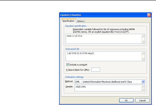
66—Chapter 20. Instrumental Variables and GMM

In the Equation specification edit box, specify your dependent variable and exogenous variables, and in the Instrument list edit box, provide a list of instruments. Endogenous variables should be entered in both the Equation specification box and the

Instrument list box.

For K-Class estimation, enter the value of k in the box labeled K (leave blank for LIML). If no value is entered in this box, LIML is performed.

If you wish to estimate a non-linear equation, then

enter the expression for the non-linear equation in the Equation specification box. Note that non-linear K-Class estimation is currently not permitted; only non-linear LIML may be performed.

If you do not wish to include a constant as one of the instruments, uncheck the Include a Constant checkbox.

Different standard error calculations may be chosen by changing the Standard Errors combo box on the Options tab of the estimation dialog. Note that if your equation was nonlinear, only IV based standard errors may be calculated. For linear estimation you may also choose K-Class based, Bekker, or Hansen, Hausman and Newey standard errors.

As an example of LIML estimation, we estimate part of Klein’s Model I, as published in Greene (2008, p. 385). We estimate the Consumption equation, where consumption (CONS) is regressed on a constant, private profits (Y), lagged private profits (Y(-1)), and wages (W) using data in the workfile “Klein.WF1”. The instruments are a constant, lagged corporate profits (P(-1)), lagged capital stock (K(-1)), lagged GNP (X(-1)), a time trend (TM), Government wages (WG), Government spending (G) and taxes (T). In his reproduction of the Klein model, Greene uses K-Class standard errors. The results of this estimation are as follows: