Appendix B. Estimation and Solution Options
EViews estimates the parameters of a wide variety of nonlinear models, from nonlinear least squares equations, to maximum likelihood models, to GMM specifications. These types of nonlinear estimation problems do not have closed form solutions and must be estimated using iterative methods. EViews also solves systems of non-linear equations. Again, there are no closed form solutions to these problems, and EViews must use an iterative method to obtain a solution.
Below, we provide details on the algorithms used by EViews in dealing with nonlinear estimation and solution, and the optional settings that we provide to allow you to control estimation.
Our discussion here is necessarily brief. For additional details, we direct you to the quite readable discussions in Press, et al. (1992), Quandt (1983), Thisted (1988), and Amemiya (1983).
Setting Estimation Options
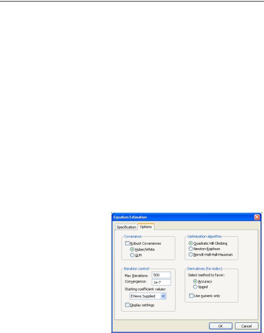
When you estimate an equation in EViews, you enter specification information into the Specification tab of the Equation Estimation dialog. Clicking on the Options tab displays a dialog that allows you to set various options to control the estimation procedure. The contents of the dialog will differ depending upon the options available for a particular estimation procedure.
The default settings for the options will be taken from the global options (“Estimation Defaults” on page 630), or from the options used previously to estimate the object.
The Options tab for binary models is depicted here. For other estimator and estimation techniques (e.g. systems) the dialog will differ to reflect the different estimation options that are available.
Starting Coefficient Values
Iterative estimation procedures require starting values for the coefficients of the model. There are no general rules for select-
752—Appendix B. Estimation and Solution Options
ing starting values for parameters. Obviously, the closer to the true values, the better, so if you have reasonable guesses for parameter values, these can be useful. In some cases, you can obtain starting values by estimating a restricted version of the model. In general, however, you may have to experiment to find good starting values.
EViews follows three basic rules for selecting starting values:
•For nonlinear least squares type problems, EViews uses the values in the coefficient vector at the time you begin the estimation procedure as starting values.
•For system estimators and ARCH, EViews uses starting values based upon preliminary single equation OLS or TSLS estimation. In the dialogs for these estimators, the drop-down menu for setting starting values will not appear.
•For selected estimation techniques (binary, ordered, count, censored and truncated), EViews has built-in algorithms for determining the starting values using specific information about the objective function. These will be labeled in the Starting coefficient values combo box as EViews supplied.
In the latter two cases, you may change this default behavior by selecting an item from the Starting coefficient values drop down menu. You may choose fractions of the default starting values, zero, or arbitrary User Supplied.
If you select User Supplied, EViews will use the values stored in the C coefficient vector at the time of estimation as starting values. To see the starting values, double click on the coefficient vector in the workfile directory. If the values appear to be reasonable, you can close the window and proceed with estimating your model.
If you wish to change the starting values, first make certain that the spreadsheet view of the coefficient vector is in edit mode, then enter the coefficient values. When you are finished setting the initial values, close the coefficient vector window and estimate your model.
You may also set starting coefficient values from the command window using the PARAM command. Simply enter the param keyword, followed by pairs of coefficients and their desired values:
param c(1) 153 c(2) .68 c(3) .15
sets C(1)=153, C(2)=.68, and C(3)=.15. All of the other elements of the coefficient vector are left unchanged.
Lastly, if you want to use estimated coefficients from another equation, select Proc/Update Coefs from Equation from the equation window toolbar.
For nonlinear least squares problems or situations where you specify the starting values, bear in mind that:
Setting Estimation Options—753
•The objective function must be defined at the starting values. For example, if your objective function contains the expression 1/C(1), then you cannot set C(1) to zero. Similarly, if the objective function contains LOG(C(2)), then C(2) must be greater than zero.
•A poor choice of starting values may cause the nonlinear least squares algorithm to fail. EViews begins nonlinear estimation by taking derivatives of the objective function with respect to the parameters, evaluated at these values. If these derivatives are not well behaved, the algorithm may be unable to proceed.
If, for example, the starting values are such that the derivatives are all zero, you will immediately see an error message indicating that EViews has encountered a “Near Singular Matrix”, and the estimation procedure will stop.
•Unless the objective function is globally concave, iterative algorithms may stop at a local optimum. There will generally be no evidence of this fact in any of the output from estimation.
If you are concerned with the possibility of local optima, you may wish to select various starting values and see whether the estimates converge to the same values. One common suggestion is to estimate the model and then randomly alter each of the estimated coefficients by some percentage, then use these new coefficients as starting values in estimation.
Iteration and Convergence Options
There are two common iteration stopping rules: based on the change in the objective function, or based on the change in parameters. The convergence rule used in EViews is based upon changes in the parameter values. This rule is generally conservative, since the change in the objective function may be quite small as we approach the optimum (this is how we choose the direction), while the parameters may still be changing.
The exact rule in EViews is based on comparing the norm of the change in the parameters with the norm of the current parameter values. More specifically, the convergence test is:
|
|
|
|
|
|
|
|
v ( i + 1 ) – v ( i ) |
|
2 |
£ tol |
(B.1) |
|
v(i) |
|
2 |
|
|
|
|
|
|
where v is the vector of parameters, 
 x
x
 2 is the 2-norm of x , and tol is the specified tolerance. However, before taking the norms, each parameter is scaled based on the largest observed norm across iterations of the derivative of the least squares residuals with respect to that parameter. This automatic scaling system makes the convergence criteria more robust to changes in the scale of the data, but does mean that restarting the optimization from the final converged values may cause additional iterations to take place, due to slight changes in the automatic scaling value when started from the new parameter values.
754—Appendix B. Estimation and Solution Options
The estimation process achieves convergence if the stopping rule is reached using the tolerance specified in the Convergence edit box of the Estimation Dialog or the Estimation Options Dialog. By default, the box will be filled with the tolerance value specified in the global estimation options, or if the estimation object has previously been estimated, it will be filled with the convergence value specified for the last set of estimates.
EViews may stop iterating even when convergence is not achieved. This can happen for two reasons. First, the number of iterations may have reached the prespecified upper bound. In this case, you should reset the maximum number of iterations to a larger number and try iterating until convergence is achieved.
Second, EViews may issue an error message indicating a “Failure to improve”after a number of iterations. This means that even though the parameters continue to change, EViews could not find a direction or step size that improves the objective function. This can happen when the objective function is ill-behaved; you should make certain that your model is identified. You might also try other starting values to see if you can approach the optimum from other directions.
Lastly, EViews may converge, but warn you that there is a singularity and that the coefficients are not unique. In this case, EViews will not report standard errors or t-statistics for the coefficient estimates.
Derivative Computation Options
In many EViews estimation procedures, you can specify the form of the function for the mean equation. For example, when estimating a regression model, you may specify an arbitrary nonlinear expression in the coefficients. In these cases, when estimating the model, EViews will compute derivatives of the user-specified function.
EViews uses two techniques for evaluating derivatives: numeric (finite difference) and analytic. The approach that is used depends upon the nature of the optimization problem and any user-defined settings:
•In most cases, EViews offers the user the choice of computing either analytic or numeric derivatives. By default, EViews will fill the options dialog with the global estimation settings. If the Use numeric only setting is chosen, EViews will only compute the derivatives using finite difference methods. If this setting is not checked, EViews will attempt to compute analytic derivatives, and will use numeric derivatives only where necessary.
•EViews will ignore the numeric derivative setting and use an analytic derivative whenever a coefficient derivative is a constant value.
•For some procedures where the range of specifications allowed is limited (e.g., VARs, pools), EViews always uses analytic first and/or second derivatives, whatever the values of these settings.